This User Guide to the JRC-DEMETRA
CGE model is intended to support basic users of the model and is
complementary to the model
documentation. It assumes that the user is familiar with the structure of
the model database, the (Walrasian) economic theory and the behavioural
relationships of the model, and CGE models implemented using the General
Algebraic Modelling System (GAMS) programming language.
In this Guide the user may find a description of the structure of the model
directory, instructions on how to calibrate JRC-DEMETRA and run comparative static
simulations. Information on more advanced applications, such as running dynamic
simulations, will be available in a second User Guide for experienced
users, under preparation.
The model is designed for calibration
using a Social Accounting Matrix (SAM), which records transactions in value
terms. In addition, JRC-DEMETRA uses two additional databases. The first
records the “quantities” of primary inputs used by each activity. If such
quantity data are not available, then the entries in the factor use matrix are
the same as those in the corresponding sub matrix of the SAM. The second set of
additional data represent the behavioural parameters employed by the model: the
elasticities of substitution for imports and exports relative to domestic
commodities, the elasticities of substitution for the CES (Constant Elasticity
of Substitution) production functions, the income elasticities of demand for
the linear expenditure system and the Frisch (marginal utility of income)
parameters for each household. All the data are accessed by the model from data
recorded in Excel and GDX (GAMS data exchange) file. All the data recorded in
Excel are converted into GDX format as part of the model program.
The User Guide refers to an
implementation of the model that uses GAMSIDE as the text editor, GDX as the
source of transactions data and destination of the model results, and Microsoft
Excel - in conjunction with GDXXRW (the utility to convert data in Excel files
to the GDX format native to GAMS) - as the source data relating to sets and
various exogenous parameters.
The master directory containing the
model code is shared with the interested user under formal request. Providing any guidance on how to
frame policy experiments using CGE models is out of the scope of this document.
All the files needed to run the model
and the experiment programs are organized within a system of directories
(Figure 1).
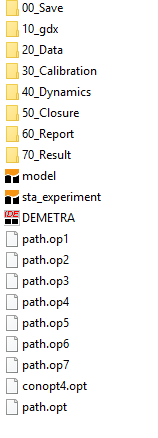
Figure 1.
Structure of the master directory
The master directory JRC-DEMETRA has
a predefined structure. Before running the model code, it contains two *.gms
program files, the *.gpr project file
and additional auxiliary files used by GAMS to run JRC-DEMETRA. All other
required files are stored within appropriate sub-directories. These files are either
“workfiles” generated during model runs, data files required for the model
calibration and INCLUDE files (bearing the .inc extension) which
help structure the model code into functional areas (e.g., reading the data,
calibrating the model, initialise variables etc.). The INCLUDE files cannot
be run independently but are invoked by the *.gms files from the master
directory.
The seven sub-directories are:
·00_Save: this folder contains two files, XXXBase.g00
and XXXBaseRef.ref, which are generated when the main model program (model.gms)
is run.
·10_gdx: as for the 00_Save folder, the
content of this folder is generated every time model.gms is run. These files generated
contain the model data in the GDX format: data_in.gdx (the database
converted from Excel into the GDX format), XXXBaseDebug.gdx (a summary
of all GAMS symbols defined in the main model program) and DEMETRA_struct_info.gdx
(a descriptive macro statistics of the economy described in the database).
·20_Data: this sub-directory contains all the
Excel files used to calibrate the model (the model database and the additional
datasets for the model calibration) and to implement comparative static and
recursive dynamic experiments (the so-called Excel experiment files).
·30_Calibration: this sub-directory contains all the
code files required to calibrate and set up the model. An important file is data_load.inc,
which contains the instructions to load the data from the Excel workbook and to
generate a GDX output file with the data converted in GDX format (data_in.gdx,
saved in the 10_gdx folder). Some of the INCLUDE files stored in
this sub-folder are used to verify the possible presence of fatal errors (e.g.,
unbalanced SAM, negative entries in the SAM). For example, samchk.inc
checks that the model is calibrated correctly by checking that the calibrated
values for variables and parameters produce balanced macro and micro-SAM. If
any of the check failed, the program aborts and reports are displayed. The code
for the model calibration is included in parmcalib_decl.inc (declaration
of all parameters required for the calibration) and parmcalib_assign.inc
(containing all calculations of parameters included in the model equations and
the base values for the model variables).
·40_Dynamics: it contains all the files needed to
run the model in its recursive dynamic version.
·50_Closure: it contains three *.inc
files defining the minimal neo-classical closure rules of the model – these
alternative closure rules are for 1) the base model runs (base.inc), 2) the
static comparative runs (static.inc) and 3) the dynamic recursive runs
(dynamic.inc). The model is thus programmed to provide a wide degree of
flexibility for the user in the selection of market clearing and model
(macroeconomic) closure rules. The supplied version of the model adopts the
principle that the model will be calibrated using a default version of these
rules (base.inc). Thereafter the user selects either the static or dynamic set
of rules for running scenarios. The user can then also alter one or more sets
of the rules depending on the assumptions they would want to consider (see the
“Running experiments” section below). These alterations can also allow the user
to conduct the same set of simulations using a range of different market
clearing and model closure rules.
·60_Report: it contains several *.inc
files that are used to generate results and macroeconomic indices, whose files
are stored in the sub-directory 70_Result.
·70_Result: This folder is populated after running
an experiment *.gms program file (e.g., sta_experiment.gms in the
above screenshot). It collects all the results in GDX format.
·90_Documentation: in this folder the user finds some
shortcuts to the latest model documentation (including that of this user guide),
stored in the JRC-DEMETRA website.
The main file for running the base
model specification is the model.gms file in the master directory. The model.gms
file is intended for the calibration of JRC-DEMETRA and for base year
replication. For scenario runs, the user should use dedicated experiment *.gms
files starting from the template provided for static simulations (sta_experiment.gms).
The model.gms file includes a series
of include commands which call the .inc files described above for
reading the model data and calibrating the model. The various include statements
in the programs require the specification of the path that identifies the
directory location of the file to be included (these paths are predefined in model.gms and therefore the user does
not need to specify them).
For an efficient way of running the
model, the JRC-DEMETRA workflow also requires the use of GAMS save and restart
facility (see more here for a more detailed description of
this GAMS feature). The facility creates the model’s workfile (*.g00) which is to be saved in the 00_save
sub-directory. This requires the user to ensure that the appropriate commands
are included in the command line area of GAMS IDE when the model program is
run. The instructions to be put in the command line are:
s=00_save\XXXBase gdx=10_gdx\XXXBaseDebug rf=00_save\XXXBaseRef
where XXX should be replaced with the
code of the country (KEN, GHA, etc.) to which the
model is calibrated. Figure 2 illustrates an example for Kenya (using the “KEN”
prefix).
![]()
Figure 2. Example of the command line
instruction in GAMS IDE.
If using GAMS Studio, the user may
also need to specify the DEMETRA working directory path through the wdir command
line option. The working directory is the location of the DEMETRA model folder
(in the example below the model is placed in C:\jrc-demetra, but this
can differ based on user preferences)
![]()
Figure 3. Example of the command line
instruction in GAMS Studio, including the working directory specification.
To assist the user in the debugging
of the model, the gdx=10_gdx\XXXBaseDebugcomponent in the above instructions makes use of the
GAMS Data Exchange facilities to record all the information relating to sets (and
alias), parameters, variables and equations present in the model code in a
single GDX file. This output GDX file is stored in the 10_gdx
sub-directory as XXXBaseDebug.gdx.
Given this method of organising and
running programs the file structures inevitably become complex and difficult to
follow. Notably for inexperienced users, it can be difficult to identify where
in the system of files symbols are declared, defined, or assigned. To help the
user in this regard, the command line is also used to generate a reference file
(XXXBaseRef.ref), using the instruction rf=00_save\XXXBaseRef that collects all this information
for the model’s symbols and identifies all the files used by the model. The
reference file can be opened in GAMSIDE and is found in the 00_Save
sub-directory (see Figure 1).
The JRC-DEMETRA program code is
contained in the file model.gms, located in the master directory
JRC-DEMETRA. Given the many procedures involved in the data loading, model
calibration and model initialization steps, the model code adopts a modular
structure. This takes the form of a series of include files that are
called from model.gms (Figure 3). In addition to the include files, the
programme requires the Excel workbook that contains the model data.
Figure 4. Overview of files included by the model.gms
main file
Model users only need to adjust the model.gms
file and the model database contained in the Excel file. The rest of the files
(the INCLUDE files) were developed to work with any model database that fits
into the requirements of the JRC DEMETRA model. The
Looking into the model.gms file
more closely, the code starts with some general information on the program, the
model description, the model terms of use and development notes.
The first group of instructions is
coded in lines 99-106 of the model.gms file (Figure 4). The command $SETGLOBAL sets the name of the control folders, located in the master directory
JRC-DEMETRA, used to store all the files needed to run model.gms and
save the model output (see Section 2). These instructions should not be changed
unless advanced users would be required to make changes to the JRC DEMETRA folder
structure.
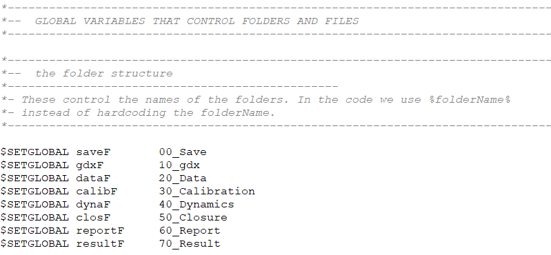
Figure 5. GAMS instructions to set up the
folder structure, model.gms main file
Good practice
Whenever the user
changes the database in the Excel file and recalibrates the model by running model.gms, it is advisable to check
whether the GDX file generated (data_in.gdx in the 10_gdx folder)
reflects the data changes. It is sometimes the case that the user does not
notice GAMS warnings flagging issues in the reading and the conversion of the
Excel file into the GDX format. In case of issues, the program could be
incorrectly using an older version of the data_in.gdx file.
Line 116 controls the database file name (.xlsx), which is the Excel data file the
program must use to calibrate the model. The program investigates the 20_Data
folder where the Excel file should be placed (Figure 5).
The next line of Figure 5 (line 117)
contains the instruction for the choice of the model’s closure rules. The
base.inc file contains the default closure rules for the base model runs.
Since model.gms is meant only for calibration and runs to ensure that
the calibration reproduces the base year, the closure rules should not impact
these aims. At the stage of running experiments (in the dedicated experiment .GMS files), the user can decide whether to choose an
alternative *.inc file from the 50_Closure folder, or to alter
these base rules explicitly within the experiment .GMS file.
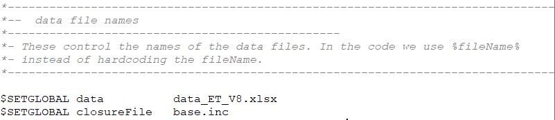
Figure 6. GAMS instructions to control the
database file name and closure rules, model.gms file
The next section of the main file
includes a list of definitions. The first group is SETS (lines 131-388), which
comprises the model sets and subsets. ALIAS are listed in lines 395-411 and are
needed when it is necessary to have more than one name for the same set.
The declaration of the model parameters follows from line 419 to 463. In the
case of JRC-DEMETRA, parameters are the model SAM and factor use datasets,
demographic and nutrition values, elasticities, and scaling parameters. Please
note that, at this stage, these model sets and parameters are only declared and
defined, not initialized.
Data are loaded with the command $INCLUDE %calibF%\data_load.inc (line 478). This data_load.inc file is in
located the folder 30_Calibration and includes all the instructions to
convert the sets of the Excel workbook to a GDX format (which will appear in
the 10_gdx folder) and then to read it in GAMS. This file also includes the
data scaling operation and initial data checks (the code of the data_load.inc
is not covered here). Further checks are done on the data by calling in the diagnost.inc
file (line 637). If there are no fatal errors and the program is not aborted,
the program proceeds with the model calibration, calling in the parmcalib_decl.inc
and the parmcalib_assign.inc files (lines 648-650).
The next step is the declaration of
the model variables (lines 669-1204). Next, to help the model reproduce the
base year with zero solver iterations, the variables are assigned initial
values to reflect the base year conditions. This is done by calling in the
varinit.inc include file (lines 1214) located in the sub-directory 30_Calibration.
Two additional files (calibCheck_decl.inc and calibCheck_assign.inc),
through a ‘calibCheck’ parameter,
help detect any differences between the variable initial (level) values and the
calibration values. Non-zero values in ‘calibCheck’ could flag some issues related
to the variable initialization or the calibration procedure.
Good practice
To ensure a successful
model calibration, the ‘iterlim’ option is important as it sets the maximum
number of iterations a solver will attempt in finding a solution to the model.
The option is normally set to a high value (e.g. 1000). When set to 0, the
solver will return infeasibilities to the model equations using the variables’
initial values set during the calibration phase. In this case, high values of
the infeasibilities (above the solver tolerance values, normally set at 10e-8)
illustrate some issues either in the Excel data used for the calibration, the calibration
process, or the equations of the model if these have been altered.
It is strongly
recommended to solve first any issues observed at this stage before moving on
to scenario analysis.
At this stage, the program carries
out further checks to be sure that the model is calibrated with a balanced SAM.
This requires the use of the samchk_decl.inc and samchk_assign.inc
files called by the program in line 1249-1251. In case of errors, the program
is aborted. Before the end of the model calibration, the program also computes
some macroeconomic and descriptive statistics of the economy under study
through the struct.inc file.
The model equations are declared
(lines 1272-1693) and then defined (lines 1704-2480). For more information on
the model equation, the user is invited to read the model documentation. Recall that the closure of model is
then determined through the inclusion of the closure file as chosen by the user
in line 117 (Figure 5).
The last section of the model.gms file contains the model
definition (the name of the model followed by the list of associated equations
to be considered by the GAMS solver). Two variants of the JRC-DEMETRA model are
included - “demetra” (lines 2521-2809) which is used for the mixed
complementarity problem (MCP) formulation of the model (the MCP formulation can
be recognized through the pairing of equations and variables through the dot
(.) operator), and “demetra_nlp” (lines 2812-2816) used for the nonlinear
program (NLP) formulation.
Following the model definitions, a
set of options for the model and the solvers are added (lines 2822–2840)
specifying the solver choice and the iteration limit among them. The ‘solve’
statement follows and includes the name of the model to be solved and the type
of problem to be considered (MCP or NLP).
JRC-DEMETRA uses two Excel workbooks, both located in the 20_Data
folder. These are employed to store the information used by the model. This
allows flexibility and replicability. The first workbook, named data*.xlsx,
contains information used for calibrating the model, while the second (experiment*.xlsx)
provides information used to run simulations. This section is concerned only with
the Excel workbook that has information used to calibrate the model (the data*.xlsx
file).
This Excel workbook is composed of several worksheets. Each
worksheet has a specific role in the model calibration, which is explained in
what follows.
It contains general information on the SAM of the country
under study. Each element of the SAM is reported by group type (e.g.,
Commodities, Activities, Factors, Households, Other accounts, and Region), with
its Code and Definition. It is important that the elements’ names
are reported correctly, to avoid the generation of errors.
It contains the Social Accounting Matrix of the country under
analysis, used to calibrate JRC-DEMETRA. The SAM must start in cell A4. Row and
column elements must be the same and reported in the Notes worksheetwith the same nomenclature.
It contains a list of all sets and parameters to be loaded by
the GAMS program (through the data_load.inc
file). Unless the user wants to pass additional data as sets and/or parameters to
the model there is no reason for the user to alter the Layout worksheet. If
changes are made to the structure of the database, it is important to ensure
that all the syntax is fully consistent. Column A identifies each element of
Column B as GAMS set or parameter. Column C defines where the element is to be
loaded from in the workbook, whilst column D and column E identify the number
of dimensions in the rows and columns of the spreadsheet.
Superset sac
The Sets worksheet contains most of the sets and
subsets used by the model. The major set of the model is sac, which
contains all the SAM accounts of the country under consideration and other
elements necessary for the model to run. Column A reports the names of the
elements and Column B the description. It is
important to ensure that the set element names are across the worksheets, if
not errors will be generated. The user needs to assign manually these subsets
when setting up an updated version of the JRC-DEMETRA model. It is a sensible
practice to copy and paste or cross-reference the subsets from the column
containing the sac account names to avoid typing errors. The JRC-DEMETRA
program will abort if the accounts names in sac and all the subsets are
not identical.
In the model.gms file,
the declaration of the sets starts in line 131. The model uses a substantial
number of subsets of sac, which are
reported under lines 146-390. The declaration of the subsets is divided by set
type (i.e., commodities, activities, factors, etc.).
The user needs to define the memberships of these subsets
manually following conventions that are obvious from the naming of the subsets.
Commodities sets
Columns J to AC
assign all commodities and/or aggregates of commodities to specific subset(s).
For example, in the subset cc Commodities and Aggregates (column J) the
user must list all commodities of the SAM (c_*) and all commodity aggregates
(c*). The latter groups are used for reporting and shocking, and the user
decides how to group the SAM commodities in this regard. For example, cagr
stands for agricultural commodities and includes all commodities of this
category. The cc set also contains the cag commodity aggregates
needed for the grouping of SAM commodities in the household utility function. Column
K contains only the commodities in the SAM (c_*).
Activities sets
The activities set is defined in
Column AF, with a functional sub-grouping of these in
sets defined in Columns AG-AQ (the same as for commodities, as described above).
For reporting purposes, the aagg set in Column AS contains a list of
commodity aggregates, which are then mapped in the model code to the activities
grouped in Columns AG-AQ.
In Column AW,
the user can define the aleon set which will comprise the list of SAM
activities for which the model will introduce a Leontief bundle at the
top-level of the corresponding production function. Therefore, the
specification of perfect complementarity of inputs at the top level must be
done here and not in the Actelast worksheet where the user needs to specify
substitution elasticities for the production functions.
Production archetypes set
Production functions are treated as
archetypes in JRC-DEMETRA. This implies that each activity will be attributed
to one user-defined archetype (e.g., “agr” for agriculture, ”liv” for
livestock, etc.). In column AT, the user needs to list the names of these
archetypes as the NT set. Each
archetype will be later be specified through the ProdNest worksheet.
Factors sets
Factors of production are listed in columns
AX-BJ. Column AZ defines the f set which
comprises the factors of production found in the SAM and considered as ‘natural
factors’. Column AY, in addition to these elements,
will comprise the so called ‘quasi factors’. These factors are specific
to the DEMETRA implementation and represent the treatment of production
intermediates (commodities) as factors of production. This is to accommodate
different assumptions on the composition of the production structure, and to allow
commodities moving from the intermediate group to the valued added group, or to
whatever branch of the production function. In such a way, they become
substitutable with production factors and can be used in the production
function as production factors. Therefore, Column AY defines the set fc which
comprises also all the commodity codes from the SAM with an f_ prefix (e.g.,
the “c_maiz” commodity will become the “f_c_maiz” quasi factor in the
production function).
Column AX defines the ff set
which is the super set of all elements included in the production functions.
The list will thus comprise natural factors, quasi factors, and the production
function bundle names (“va” for the value-added bundle, “flab” for the labour bundle, etc.). These
last elements are defined in the fag set (Column BA)
and will be used in the ProdNest worksheet to specify how natural factors and
quasi factors are bundled in the production function nesting of each production
archetype.
The content of columns BB-BH comprise
a grouping of factors that are SAM-specific. The grouping of factors is useful,
in the equation definition, for reporting and shocking the model. Of these,
columns BB and BF
cannot be left empty and must include the list of labour factors and capital factors,
respectively.
Institutions sets
Columns BK-BN comprise the grouping
of institution accounts present in the SAM (household groups, enterprise,
government, trade partners – one or several). For households, Column BO also determines the accounts that belong to the
rural areas (the hrur set).
Column BP
defines the set g associated to the government and the tax accounts.
Column BQ comprises defines the gt set with just the tax accounts as
elements.
Columns BS
and BV define the enterprise account and the trade
partners accounts, respectively.
Column BT
defines the investment-savings account, set i. Note that the model can
accommodate multiple accounts in this set, in case investment needs to be
broken down into different typologies.
Column BX together with Column BY
define the list of households and their associated factors that can enter the migration
equations of the model.
Other sets
Of the remaining columns in the Sets worksheet, Columns CB
and CD are important since they define commodities
associated with the educational spending and health spending, respectively. These
sets (ceduc anc cheal) enter the model equations.
Column CP
defines the reg set which list the geographical regions that are present
in the SAM data. The mapping of these regions to actual activities and
households is done in the Maps worksheet.
The rest of the sets are for
reporting purposes and are self-explanatory. Leaving these sets blank will not
have an impact on the model.
In several calibration statements and
equations, it is necessary to match data that are recorded using slightly
different but related labels. This requires the provision of a series of
mapping sets that define the matching of set elements. These mapping sets
(recognizable as multi-dimensional sets) are defined in the Maps worksheet.
The user needs to compile this
worksheet to ensure the structure of the model is according to the needs of the
analysis. The most relevant ones are those related to the production function -
map_NT_a, map_fag_NT_leo and map_f_c and that related to the household
demand system grouping map_cag_c.
Production function definition mapping
Through map_NT_a (Columns Y-Z)
the activities in the model are mapped to specific production function
archetypes (as listed in the NT set in column AT of the Sets worksheet). The map_f_c set (Columns AA-AC)
ensures the mapping between commodities, quasi-factors f_c and
production function archetypes. The user would thus need to list the conversion
to a quasi-factor for each intermediate input and for each production archetype
NT. The map_fag_NT_leo set (Columns AM-AN) specifies the production
bundles fag (defined in Column BA in the Sets worksheet) to be treated as Leontief nests in
specific production function archetypes NT.
Household demand system definition mapping
Through map_cag_c (column AB) the user should specify how market and home
commodities present in the SAM (defined by the c set) are to be grouped
for an LES-CES demand system.
map_cag_c will thus include an assignment off all cces elements
to one cles element. Once completed, the user will also need to specify
the income and substitution elasticities for each household group – see
explanations below for the hoelast and hocelast sheets.
If the user decides to use a simpler LES
(Linear Expenditure System) demand system (the base implementation DEMETRA SAMs), then the cces set will be empty, while
the cles will contain all home and market commodities which are part of
the c set. In this case map_cag_c will also be empty.
Other important mappings
The user will also need to specify
the import and export tax accounts mapping to individual trade partner. As JRC
DEMETRA allows for multiple trade partners, there would be an import tax and an
export tax SAM account for each. The mapping of these is to be specified
through map_mtax_w (Columns AH-AI) for import tax accounts and through
map_etax_w (Columns AK-AL).
Another important set is map_a_c
(Column BC) which maps the activities having as
output an HPHC commodity. With activities defined by region and commodities
defined nationally, the set will include multiple activities producing the same
national commodity.
The worksheet will contain other mapping
sets used for reporting purposes.
The worksheet contains a three-dimensional matrix defining
the bundling in the structure of the production function archetypes (defined in
the NT set in column AT in the sets sheet). The matrix is
presented with two dimensions by row (production archetype NT in Column
B and production factors ff in Column C) and one dimension by column
(production bundle fag on row 6). Note that the factors include the
entire ff set which comprises natural factors, quasi-factors, and
aggregate factors (production bundles).
The data is read by the model.gms
file starting from cell B6 downwards and rightwards. Column A is just for
cross-checking if the factor names introduced are part of the ff set defined in
the Sets worksheet Column AX.
The matrix is filled in by specifying “1” for the presence of
a factor ff under a specific production bundle. This is to be specified
for each production archetype NT. Note that each active row of the matrix needs
to have one and only one “1” marked. The list of ff factors also needs to be
exhaustive (all factors and active aggregate should be listed for each production
archetype). In this regard, column N is just for checking the attribution of an
ff factor to a specific production bundle – for a correct specification,
all elements should be “1” in this column.
Column S controls that each element listed in column C enters
a bundle of row 6 only once.
There are numerous aspects of the model structure and the
flow of the program that the user might wish to control. The approach used in
the JRC-DEMETRA model is to concentrate these aspects of the program Controls
worksheet. This has two tables of entries.
The first, “mod_control,” contains several elements that pass
parameters to the model that control aspects of model structure. The values in
this block condition the model. They control:
a) "numerchk” – checking for the model homogeneity if
value other than 1;
b) “minaqxsh” - minimum intermediate input share for the top-level
production function to be a CES bundle;
c) “samscal”-
starting scaling factor value for operation of automatic scaling;
d) “scaltarg” - target upper value for SAM entries after
scaling;
e) “scalprop” - proportion of non-zero elements that must be
below the target level;
f) “setpop” - deprecated
g) “toldiffsam” - tolerance for difference between SAM
account totals on rows and columns;
h) “mincetsh” - deprecated
e) selection of elasticity values;
f) number of trade nests in ARM
and CET functions.
The second, “flow_control,” passes parameters to the model
that are used to determine whether various IF statements are
implemented, and whether certain non-crucial components of the program run.
Most of these actions are needed when setting up a new version or when
modifying the model. Specifically, they control:
a) display of data and sets;
b) display of parameters;
c) display of initial variable values;
d) export of base data to GDX;
e) export of ALL sets, data, parameters etc., to GDX.
The flow controls are 1/0 parameters. If the parameter has a
value of “1” then an action is implemented and if its value is “0” it is not
implemented. Generally, the flow control parameters determine whether an IF statement
is implemented or not. When a statement is implemented, it typically controls
output, either by running an INCLUDE file that produces output or
implementing a display or export command in GAMS.
In this worksheet the value data in
the SAM can be converted into quantity data. For example, the user can specify how
many employers or how many number of hours of work were employed by each activity
account in the SAM. If the user does not have this information, they can
instruct the same numbers in this sheet as those in the SAM. In this case the factuse
will capture a quantity of factor use equal to the SAM value and thus the return
wages will be equal to one in the calibration phase. However, changing the
factuse values to reflect physical quantities obtained (from e.g., labour
surveys) will allow the model to calibrate the wage levels per unit of factor
use (for instance, hour of work for labour or hectare for land) but also to
account for differences in rents and wages across activities. In this way,
users can assign heterogenous rate of return to apparently homogenous factors.
This worksheet contains information
about initial unemployment rates of each factor, if relevant. In this case, factor
supply would be endogenous and the return to the factor fixed. If this
worksheet is left empty, the closure rule of the model is full employment of
all factors.
If the user has information about demographic parameters, like death and birth rates, and elasticities this is the dedicated worksheet. The elasticities are the link between spending on education and health and labour productivity, the link between education and birth rate, and the link between investment in health and impact on death rate.
In addition to the transactions data derived from the
(aggregate) SAM the model also needs a series of elasticities, which must be
exogenously assigned by the user. This is the worksheet where the model
specific commodity elasticities are reported. The sigma elasticity
drives the substitution between imported and domestic commodities to meet
domestic demand. The omega elasticity defines how quickly the producer changes
from domestic to export market, given a change in the relative price.
The elasticities contained in this
worksheet measure the percentage change in the inputs used in the production
process in response to a percentage change in their prices.
The elasticity of substitution
between factors in production relates the change in the ratio of factors used
in a production process to a given change in the factor price ratio. For each
nest of the production tree (represented by aggregate factors fag in column C) and for each
activity in the SAM (in row 5) an elasticity of substitution needs to be
assigned. Therefore, additional entries would be required if the production
function is elaborated by the user through changes in composition of the
elements of the fag set (for instance,
introducing new production function bundles requiring new elements in the fag
set) and changes in the production function definition through the prodNest
sheet
This worksheet contains the income
elasticity of households by household commodity group (defined by the cag set in column AB in the sets sheet). It measures how responsive
the quantity demanded for a good or service is to a change in household income.
This worksheet contains the elasticities
of substitution in the LES-CES demand system. The user needs to specify the CES
elasticity value for each element of the cag set and for each activity.
The Frisch parameter is the
substitution parameter measuring the sensitivity of the marginal utility of
income to income/total expenditures. This parameter is crucial in the
calibration process of CGE models that adopt LES demand systems, like DEMETRA.
It must be exogenously assigned by the user.
This worksheet contains information
on the nutritional intake (calories, proteins, and fat) of agricultural
commodities.
The sheet contains a 4-dimensional matrix with two dimensions
on the columns and two on the rows. The two dimensions on the rows define the
factor-household combinations from which the migration originates, while the
two dimensions on the columns define the factor-household combination for the
destination. Placing a value within the matrix will thus define the migration
elasticity between source and destination, ensuring that with migration,
households also bring along their factors of production. An absent or zero
value prevents any migration between that specific source and destination pairs
to take place. For how the migration elasticities enter the model structure,
the user is referred to the “Household Migration and Factor Mobility” section
of model documentation.
The JRC-DEMETRA model has several aspects that facilitate
checking that the model is correctly specified. Whenever the user makes any
changes to the model or the model data these checks should be conducted BEFORE
carrying out any simulations; failure to do so may mean that the simulations
are conducted using an incorrectly specified model.
·Walras
check. Look for the variable “Walras,” it should equal zero, or very nearly zero.
·Check
the Left-hand sides: search for ‘LHS,’ then after finding the first occurrence
of ‘LHS’ search for ‘***.’ If any equations are incorrectly specified, they are
identified.
·Check
data replication: first check the Macro SAM: search for ‘ASAMG2CHK’ – all the
values should equal 1; then search for and check DIFFASAMG2 and CNTASAMG2 –
these should be zeros or close to zero. Second check the Micro SAM: search for
and check DIFFSAMG2 and CNTSAMG2 – these should be zeros or close to zero.
·Check
if the model is homogeneous. JRC-DEMETRA is a real model, the results must be
independent from prices. Run a numéraire check. In the Excel workbook go to the
Controls worksheet and change the value of ‘numerchk’
to 2, save the Excel file and rerun the model. Then check the Macro SAM: search
for ‘ASAMG2CHK’ – all the values
should equal 2.
If the model passes all these checks, the model will
(usually) be correct.
When the model passes all the above
checks, the next step of the workflow is running comparative static simulations.
To this purpose, the user needs a second *.gms file, called sta_experiment.gms,
located in the master directory JRC-DEMETRA (Figure 1). The model calibration
is done only once unless the user changes something in the Model Excel Workbook
(Figure 6). The calibration is passed on to the experiment file through the
model workfile, XXXBase.g00, located in the 00_Save folder.
To run any static simulation, the
user must compile an Experiment Excel Workbook called experiment_XXX.xlsx and
located in the 20_Data folder of the
main directory. This Excel Workbook contains the characteristics of the
simulation and any additional data needed to run it. At the end of the experiment,
the script generates a set of result files, stored in the 70_Results folder (Figure 6).
In addition, the user needs to load the model workfile
through the GAMS restart feature and to include other useful options for
running the model. This is done by entering the following options in the
command line of GAMS IDE:
r=00_save\XXXBase
s=00_save\XXXExp gdx=10_gdx\XXXExpDebug rf=00_save\XXXExpRef
where XXX should be replaced with the country 3 letter code
(e.g. KEN for Kenya). Examples of this string for different countries are
available in lines 7-11 of the sta_experiment.gms
file. If using GAMS Studio, the additional wdir option could be needed to indicate the working
directory of the DEMETRA model, in the same way as for running the model.gms file.
Running dynamic
simulations
As reported in the
technical documentation, the DEMETRA framework can also run recursive dynamic
simulations. Recursive dynamic applications all start from the respective
comparative static models, by exploiting the LOOP facility provided by GAMS, so
that the recursive dynamic applications operate as series of comparative static
simulations where the ‘dynamic’ updates are implemented between each
comparative static simulation. However, as pointed out in the Introduction,
providing instructions on how to run dynamic simulations with JRC-DEMETRA is
out of the scope of this Guide. Users interested in running the model in a
recursive dynamic setup should contact the DEMETRA JRC team.
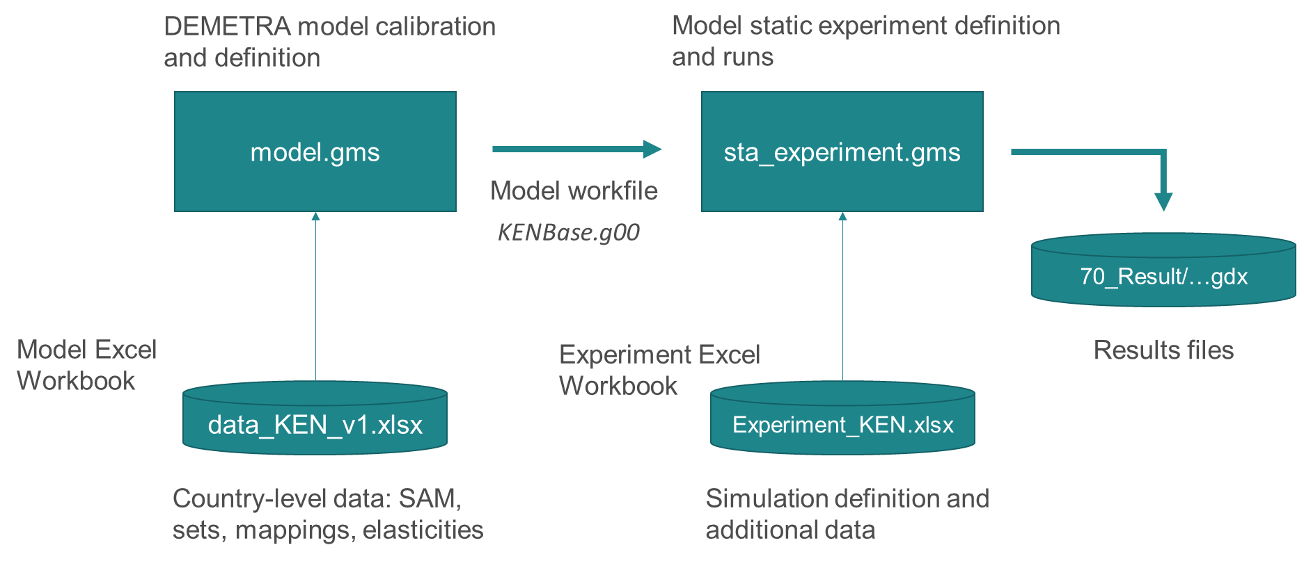
Figure 7: Workflow of running JRC-DEMETRA.
As for the model.gms file, the experiment GAMS code adopts a modular
structure. This takes the form of a series of include files that are
called from sta_experiment.gms (Figure 7). In addition to the include
files, the programme requires the Experiment Excel Workbook that contains all
the additional information required to run simulations. This excel workbook is called
in line 18 of the *.gms file and located
under the 20_Data folder.

Figure 8: Overview of files included by the sta_experiment.gms file.
As can be seen in Figure 7, the sta_experiment.gms file for
static comparative simulations allows for a set of simulations to be run
sequentially. This is ensured through a GAMS “loop” statement which iterates
over all simulations sim1 included in
the Experiment Excel Workbook (see Compiling the Experiment Excel
Workbook)
With the completion of each simulation the level values for
the results are assigned to the appropriate results parameter – all results
parameters use the same name as the associated variable but prefixed with ‘res.’
These levels results are subsequently used to derived additional (analytical)
results, stored in 70_Results folder. See more in Navigating the simulations results.
The base distribution of the DEMETRA model will include a
series of files as Experiment Excel Workbooks tailored to the accounts used in
the SAMs also included in the /20_Folder. These country-specific workbooks
(experiment_XXX.xlsx) serve as templates and should not be modified. For each
new set of simulations, the user should instead open the workbook of the
relevant country and save this under a different name to reflect the label of
the intended analysis.
The structure of the Excel workbooks for experiments is similar
to the model data, where a shorter series of worksheets contain most of the
relevant information to set up the model runs for a set of simulations. For
simplification purposes, this file also contains the information needed when
the user wishes to run dynamic
simulations (in ‘macro’ and ‘dyn_data’ sheets). Except for changes to the
series of closure rules, which the user can make by selecting an alternative
closure file (the default is base.inc) or by manually specifying specific
closures for individual simualtions, the changes applied during the experiment
stage cannot affect the behavioural structure of the model.
This sheet contains all the elements listed in the other worksheets;
therefore, it is important to ensure that all the syntax is fully consistent. Column
A identifies each element of Column B as GAMS set or parameter. Column C
defines where the element is to be loaded from in the workbook, whilst column D
and column E identify the number of dimensions in the rows and columns of the
spreadsheet.
It contains the simulation sets, grouped as follows:
·Sim: all simulation sets (column A)
with description (column B);
·Sim1: applied simulation sets (column C) with description (column
D). Column D sim1 is the set of simulations that GAMS will run. It is useful
when the user wants to focus on specific scenarios. Changing the membership of
this set allows for the running of different combinations of shock. The sim1 elements are a subset of sim, therefore any element in sim1 should also appear in sim, otherwise running sta_experiment.gms will end up returning
an error.
·Simr: reported simulations set –
deprecated
For static simulations, both sim and sim1 should at
least comprise a “Base” element which is the baseline simulation. Result values
from this simulation will be used to calculate changes from baseline of the
policy-specific simulation declared and implemented by the user. The “BaU”
element is not used in comparative static runs but only in the dynamic
recursive ones.
Figure 9: Simulation sets worksheet.
This worksheet contains a range of sets and mappings useful for the aggregation of results in various forms such as by macro activities, region or urban/rural. Unless the account names of the underlying SAM do not change, the user does not need to modify anything in this worksheet.
This worksheet contains a range
of sets useful for the results reporting script of the DEMETRA framework. Users
should not modify these as they are general for all countries and simulations.
- deprecated
Can be useful to input data for recursive dynamic
simulations.
Before anything, the user should save the sta_experiment.gms file under a different desired name, reflecting the name of the analysis. Once this done and the newly saved file is open, the user can add specific details of the intended simulations set. In section 1 of this file, at line 18, the user can indicate the name of the Experiment Excel Workbook created as detailed above. The name should also include the “.xlsx” extension of the file.
Next, the user can indicate some labels to be attached to the experiment – these labels will then be reflected in the name of the results .gdx files created after the simulations are completed. The first label is Mode and is set by default as “sta” (for static), therefore, the user may want to keep it as such for all static simulations. The next label is exp which the user can use to further detail the nature of the simulations set. If choosing a multi-word label, a good practise is to use an underscore “_” character to replace the space between words (for example, “VAT_reform”).
For the simulations set sim declared in the Experiment Excel Workbook, a series of simulation GAMS parameters (referred to here as ‘simulation containers’) are declared in sta_experiment.gms in lines 81-208. Examples of some of these containers are included in Figure 9. As can observed, these containers bear the same name as parameters of variables entering the DEMETRA model equations, having the suffix “SIM”. For instance, TEADJSIM(w,sim) is linked to the TEADJ export subsidy scaling factor in equation (GT2) (see model documentation). By default, these containers are initialised in lines 214-317 (in sta_experiment.gms) with the base values also used during the calibration stage of the DEMETRA model.
To apply specific shocks, in a first step, the user can use these simulation containers to store the shock values for individuals simulations belonging to the sim set. This is done in section 2b in sta_experiment.gms (line 320). In the example below TEADJSIM is assigned value 0.5 across all commodities c for the “test” simulation (assuming “test” was declared in the simsets sheet of the Experiment Excel Workbook).

Up to this point, only applying values to the simulation containers will not produce any effects when running the model as these simulation containers are not part of the model equations. Therefore, a second step is required to transfer the shock values from the simulation containers to model parameters and variables. This is done in section 7 of the sta_experiment.gms (line 360) which is placed within the GAMS loop going through the sim1 simulation set. For each element of sim1 (as declared in the Experiment Excel Workbook) the relevant model components are updated. In the example below, the TEADJ model parameter is updated with the value from the simulation container TEADJSIM.
Once values are transferred, a solve statement follows in the same GAMS loop, in section 8 of the experiment GAMS file. A few options are included, among which the solvers to be used for the MCP and NLP model formulations.

After this user interventions, the simulation .gms file is ready to be run.
The DEMETRA framework offers a reporting script which
produces a set of results files saved as .gdx
files in the /70_Result folder. As
depicted in Figure 7, the reporting script is by default integrated within the
simulation workflow, therefore, it does not require any additional user
actions. The script will produce the following .gdx files, where yyy is the “exp” label set by the user when initialising the experiment GAMS file:
·sta_yyy_resLevel.gdx – contains the level values of most
model variables across all applied simulations included in the Experiment Excel
Workbook. This also captures the values for the Baseline (“Base” simulation). Associated
is sta_yyy_resLevelAggr.gdx containing the level values aggregated
according aggregation mappings from the Experiment Excel Workbook.
·sta_yyy_resDiffBase.gdx – contains the level difference of simulations from the
Baseline.
·sta_yyy_resPerBase.gdx – contains the percentage difference
of simulations from the Baseline. Associated is sta_yyy_resPerBaseAggr.gdx
containing the aggregate percentage differences based on aggregation mappings.
·sta_yyy_resmacro.gdx – contains macro totals (components of GDP and others)
calculated post-simulation. These are expressed in both nominal and real terms.
·sta_yyy_reswelf.gdx – contains welfare metrics such as Equivalent Variation values resulting
from the applied simulation
·sta_yyy_resstruct.gdx – contains information over economic structural changes
occurring through the applied simulations. These changes can refer to
expenditure, demand, trade and factor use.