This document provides a description of the Dynamic Equilibrium Model for Economic development Resources and Agriculture (DEMETRA) single-country computable general equilibrium (CGE) model. DEMETRA is a development of the STAGE_DEV models documented in (McDonald et al., 2016). STAGE_DEV is a variant of STAGE_2 (McDonald, 2015) that incorporates a series of additional behavioural relationships that better account for economic relationships in developing countries, such as the dual role of semi-subsistent agricultural households, a nested consumption function, the endogeneity of the functional distribution of income, domestic migration and factor market segmentation. The recursive dynamic version of DEMETRA is derived from the STAGE_DYN model and STAGE_DEV_DYN models. that is a variant/development of the STAGE 2 single country CGE model. Recursive dynamic applications of the STAGE family of CGE models all start from the respective comparative static models, by exploiting the LOOP facility provided by GAMS (General Algebraic Modelling System), so that the recursive dynamic applications operate as series of comparative static simulations where the ‘dynamic’ updates are implemented between each comparative static simulation. Thus, an in-depth understanding of the comparative static versions of the model is essential before progressing to the recursive dynamic versions.
The core model is extended with the inclusion of multipartner trade, a fully flexible production function and other changes documented in this document.
The model is agnostic with respect to macroeconomic closure and market clearing conditions and is coded so as to allow the user substantial degrees of freedom to impose different views on how an economy operates. The models also include a substantial number of variables included so as to simplify the coding of adjustments needed for experiments; by and large these adjustment instruments use a standard formulation.
The model is designed for calibration using a reduced form of a Social Accounting Matrix (SAM) that broadly conforms to the UN System of National Accounts (SNA). Table 1 contains a macro SAM in which the active sub matrices are identified by X and the inactive sub matrices are identified by 0. In general, the model will run for any SAM that does not contain information in the inactive sub matrices and conforms to the rules of a SAM. In some cases a SAM might contain payments from and to both transacting parties, in which case recording the transactions as net payments between the parties will render the SAM consistent with the structure laid out in Table 1.
The most notable differences between this SAM and one consistent with the SNA are:
1) The SAM is assumed to contain only a single ‘stage’ of income distribution. However, transforming the functional distribution of income using apportionment (see Pyatt, 1989) will render the SAM consistent.
2) A series of tax accounts are identified (see below for details), each of which relates to specific tax instruments. Thereafter a consolidated government account is used to bring together the different forms of tax revenue and to record government expenditures. These adjustments do not change the information content of the SAM, but they do simplify the modeling process. However, they do have the consequence of creating a series of reserved names that are required for the operation of the model.
The model contains a section of code, immediately after the data have been read in, that resolves a number of common ‘issues’ encountered with SAM databases by transforming the SAM so that it is consistent with the model structure without any marked loss of information. Specifically, all transactions between an account with itself are eliminated by setting the appropriate cells in the SAM equal to zero. Second, some transfers from domestic institutions to the Rest of the World and between the Rest of the World and domestic institutions are treated net as transfers to the Rest of the World and domestic institutions, by transposing and changing the sign of the payments. And third, some transfers between domestic institutions and the government are treated as net and as payments from government to the respective institution. Since these adjustments change the account totals, which are used in calibration, the account totals are recalculated within the model.
Table 1 Macro SAM for the Standard Model
|
|
Commodities |
Activities |
Factors |
Households |
Enterprises |
Government |
Capital Accounts |
RoW |
|
Commodities |
0 |
X |
0 |
X |
X |
X |
X |
X |
|
Activities |
X |
0 |
0 |
0 |
0 |
0 |
0 |
0 |
|
Factors |
0 |
X |
0 |
0 |
0 |
0 |
0 |
X |
|
Households |
0 |
0 |
X |
0 |
X |
X |
0 |
X |
|
Enterprises |
0 |
0 |
X |
0 |
0 |
X |
0 |
X |
|
Government |
X |
X |
X |
X |
X |
0 |
0 |
X |
|
Capital Accounts |
0 |
0 |
X |
X |
X |
X |
0 |
X |
|
RoW |
X |
0 |
X |
X |
X |
X |
X |
0 |
|
Total |
X |
X |
X |
X |
X |
X |
X |
X |
In addition to the SAM, which records transactions in value terms, two additional databases are used by the model. The first are two satellite accounts that record the ‘quantities’ of primary inputs used by each activity and the quantities of factors owned by each institution. If such quantity data are not available, then the entries in the factor use and ownership matrices are the same as those in the corresponding sub matrices of the SAM. The second series of additional data are the elasticities of substitution for imports and exports relative to domestic commodities, the elasticities of substitution for the CES production functions, the income elasticities of demand for the linear expenditure system and the Frisch (marginal utility of income) parameters for each household, and factor mobility and household migration elasticities.
All the data are accessed by the model from data recorded in Excel and GDX (GAMS data exchange) file. All the data recorded in Excel are converted into GDX format as part of the model.
A key design principle of the model is that it is a ‘template’ model. In this case the term ‘template’ is defined as meaning that the model has been compiled with the expectation that users of the model are likely to, and/or should, make changes to the model so as to customise the model to the specific circumstances of the economy being studied and/or the policy issues be simulated.
The developers of and contributors to this model are supportive of users who extend the model and hope that such users will share their efforts with other users.
The model uses a series of sets, each of which is required to be declared and have members assigned. For the majority of the sets the declaration and assignment takes place simultaneously in a single block of code. However, the assignment for a number of the sets, specifically those used to control the modeling of trade relationships is carried out dynamically by reference to the data used to calibrate the model. The following are the basic sets for this model

and for each set there is an alias declared that has the same membership as the corresponding basic set. The notation used involves the addition of a ‘p’ suffix to the set label, e.g., the alias for c is cp.
However, for practical/programming purposes these basic sets are declared and assigned as subsets of a global set, sac,
![]()
All the dynamic sets relate to the modeling of the commodity and activity accounts and therefore are subsets of the sets c and a. The subsets are
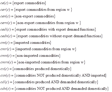
and members are assigned using the data used for calibration. Additionally there are some sets, referring to commodities and activities, which are used to control the behavioural equations implemented in specific cases. These are
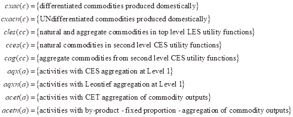
and their memberships are set during the model calibration phase.
Finally a set is declared and assigned for a macro SAM that is used to check model calibration. This set and its members are
![]() .
.
The model also uses a number of names that are reserved, in addition to those specified in the set statements detailed above. The majority of these reserved names are components of the government set; they are reserved to ease the modeling of tax instruments. The required members of the government set, with their descriptions, are
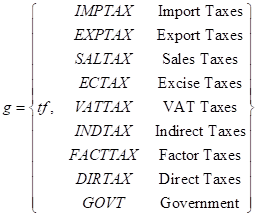
where tf is the set of factor use taxes, with one member of tf for each member of the set of factors, f.
The other reserved names are for the factor account and for the capital accounts. For simplicity the factor account relating to residual payments to factors has the reserved name of GOS (gross operating surplus); in many SAMs this account would include payments to the factors of production land and physical capital, payments labeled mixed income and payments for entrepreneurial services. Where the factor accounts are fully articulated GOS would refer to payments to the residual factor, typically physical capital and entrepreneurial services.
The capital account includes provision for multiple expenditure accounts relating to investment. All expenditures on stock changes are registered in the account dstoc, while all investment expenditures are registered to investment accounts k**. All incomes to the capital account accrue to the i_s account and stock changes are funded by an expenditure levied on the i_s account to the dstoc account.
The equations for the model are set out in eleven ‘blocks’; which group the equations under the following headings ‘trade’, ‘commodity price’, ‘numéraire’, ‘production’, ‘factor’, ‘household’, ‘enterprise’, ‘government’, ‘kapital’, ‘foreign institutions’ and ‘market clearing’. This grouping of equations is intended to ease the reading of the model rather than being a requirement of the model; it also reflects the modular structure that underlies the programme and which is designed to simplify model extensions/developments.
A series of conventions are adopted for the naming of variables and parameters. These conventions are not a requirement of the modeling language; rather they are designed to ease reading of the model.
• All VARIABLES are in upper case.
• The standard prefixes for variable names are: P for price variables, Q for quantity variables, E for expenditure variables, Y for income variables, and V for value variables
• All variables have a matching parameter that identifies the value of the variable in the base period. These parameters are in upper case and carry a ‘0’ suffix, and are used to initialise variables.
• A series of variables are declared that allow for the equiproportionate adjustment of groups of parameters. These variables are named using the convention **ADJ, where ** is the parameter series they adjust.
• All parameters are in lower case, except those used to initialise variables.
• Names for parameters are derived using account abbreviations with the row account first and the column account second, e.g., actcom** is a parameter referring to the activity:commodity (supply or make) sub-matrix;
• Parameter names have a two or five character suffix which distinguishes their definition, e.g., **sh is a share parameter, **av is an average and **const is a constant parameter;
• The names for all parameters and variables are kept short.
Trade relationships are modeled using the Armington assumption of imperfect substitutability between domestic and foreign commodities and among different trade partners. The set of equations are split across two sub-blocks – exports and imports - and provide a general structure that accommodates most eventualities found with single country CGE models. In particular, these equations allow for traded and non-traded commodities while simultaneously accommodating commodities that are produced or not produced domestically and are consumed or not consumed domestically and allowing a relaxation of the small country assumption of price taking for exports.
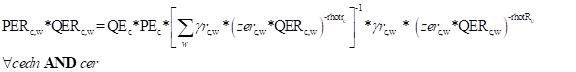
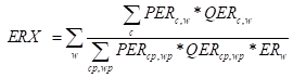
The domestic price of exports from a specific region (E1) is defined as the product of the world price of exports (PWE), the exchange rate (ER) and one minus the export tax rateand are only implemented for members of the set c that are exported, i.e., for members of the subset ce. The cost of transporting commodities in the form of prices of per unit margin services are also included in determining PERc. The world price of imports and exports are declared as variables to allow relaxation of the small country assumption, and are then fixed as appropriate in the model closure block. E2 employs an index to calculate the aggregate export price PE from all bilateral partners.
The output transformation functions (E3), and the associated first-order conditions (E5), establish the optimum allocation of domestic commodity output (QXC) between domestic demand (QD) and exports (QE), by way of CET functions, with commodity specific share parameters (g), elasticity parameters (rhot) and shift/efficiency parameters (at). The equation also include a shift parameter ze, which allows to exogenously modifying the preference between domestic sold and exports. The first order conditions (E5) define the optimum ratios of exports to domestic demand in relation to the relative prices of exported (PE) and domestically supplied (PD) commodities. But (E3) is only defined for commodities that are both produced and demanded domestically (cd) and exported (ce). Thus, although this condition might be satisfied for the majority of commodities, it is also necessary to cover those cases where commodities are produced and demanded domestically but not exported, and those cases where commodities are produced domestically and exported but not demanded domestically.
An additional Armington Equation (E4) allocate export to different bilateral partners in case the database allows for multiple trade partners. E4 establishes the optimum allocation of exports (QE) to each partners (QER), by way of CET functions, with commodity specific share parameters (gr), elasticity parameters (rhotr)). The equation also include a shift parameter zer which allows to exogenously modifying the preference among different partners.
![]() (E1)
(E1)
 (E1B)
(E1B)
 (E2)
(E2)
![]() (E3)
(E3)
![]() (E3b)
(E3b)
 (E4)
(E4)
 (E5)
(E5)
![]() (E5b)
(E5b)
![]() (E5c)
(E5c)
![]() (E5d)
(E5d)
![]() (E6)
(E6)
 (E7)
(E7)
If commodities are produced domestically but not exported, then domestic demand for domestically produced commodities (QD) is, by definition (E6), equal to domestic commodity production (QXC), where the sets cen (commodities not exported) and cd (commodities produced and demanded domestically) control implementation. On the other hand if commodities are produced domestically but not demanded by the domestic output, then domestic commodity production (QXC) is, by definition (E6), equal to commodity exports (QE), where the sets ce (commodities exported) and cdn (commodities produced but not demanded domestically) control implementation.
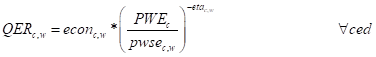
The equations E1 to E6 are sufficient for a general model of export relationships when combined with the small country assumption of price taking on all export markets. However, it may be appropriate to relax this assumption in some instances, most typically in cases where a country is a major supplier of a commodity to the world market, in which case it may be reasonable to expect that as exports of that commodity increase so the export price (PE) of that commodity might be expected to decline, i.e., the country faces a downward sloping export demand curve. The inclusion of export demand equations (E7) accommodates this feature, where export demands are defined by constant elasticity export demand functions, with constants (econ), elasticities of demand (eta) and prices for substitutes on the world market (pwse).
The domestic price of competitive imports for a given trade partner (M1) is the product of the world price of imports (PWM), the exchange rate (ER) and one plus the import tariff rate (TMc,w). These equations are only implemented for members of the set c that are imported, i.e., for members of the subset cmr. The domestic price of competitive imports (M2) is the sum of all bilateral imports values(PMR*QMR) divided by the quantity of competitive imports (QM).
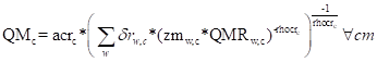
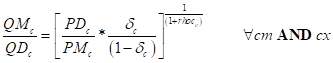
The domestic supply equations are modeled using Constant Elasticity of Substitution (CES) functions and associated first order conditions to determine the optimum combination of supplies from domestic and foreign (import) producers. The domestic supplies of the composite commodities (QQ) are defined as CES aggregates (M3) of domestic production supplied to the domestic market (QD) and imports (QM), where aggregation is controlled by the share parameters (d), the elasticity of substitution parameters (rhoc) and the shift/efficiency parameters (ac). The equation also include a shift parameter zm, which allows to exogenously modifying the preference between domestic produced and imported goods. The first order conditions (M3) define the optimum ratios of imports to domestic demand in relation to the relative prices of imported (PM) and domestically supplied (PD) commodities. But (M6) is only defined for commodities that are both produced domestically (cx) and imported (cm). Although this condition might be satisfied for the majority of commodities, it is also necessary to cover those cases where commodities are produced but not imported, and those cases where commodities are not produced domestically and are imported.
![]() (M1)
(M1)
![]() (M2)
(M2)
![]() (M1b)
(M1b)
![]() (M2b)
(M2b)
 (M3)
(M3)
![]() (M4)
(M4)
 (M5)
(M5)
 (M6)
(M6)
![]() (M6b)
(M6b)
![]() (M6b)
(M6b)
![]() (M6c)
(M6c)
![]() (M7)
(M7)
If commodities are produced domestically but not imported, then domestic supply of domestically produced commodities (QD) is, by definition (M4), equal to domestic commodity demand (QQ), where the sets cmn (commodities not imported) and cx (commodities produced domestically) control implementation. On the other hand if commodities are not produced domestically but are demanded on the domestic market, then commodity supply (QQ) is, by definition (M7), equal to commodity imports (QM), where the sets cm (commodities imported) and cxn (commodities not produced domestically) control implementation.
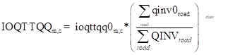
Trade and transport margins – margin services - record the costs of transferring commodities from their source (factory gate and port of entry) to consumer (domestic or foreign). At their sources commodities are valued at basic prices while at the point of consumption they are valued at purchaser prices, i.e., inclusive of indirect taxes and trade and transport margins. The key assumption is that trade and transport margins are represented by the quantity of trade and transport services required to deliver a unit of the commodity to the consumer (IOQTTQQ and ioqttqe – for supplies to the domestic and foreign consumers respectively). Thus the quantity of trade and transport services required by the economy (QTT) is defined by the quantity of commodities demand times the quantity of margin services per unit of delivered commodity (M2).
The quantities of the commodities required (QTTD) to produce a unit of margins services are defined by Leontief technologies where the input coefficient (ioqtdttc,m) define the quantities of commodity c required to produce a unit of the margin services m (M3). Given the Leontief technologies the unit cost of the margin services (PTT) is a simple weighted average of the costs of the commodities used in its production (M1).
The change of the quantity of trade and transport services required to deliver a unit of the commodity to the consumer for supplies to the domestic (IOQTTQQ) depends on the variations of investment in sectors which increase transportation infrastructure (road) based on a given elasticity (etatr) (M4).
![]() (M1)
(M1)
![]() (M2)
(M2)
![]() (M3)
(M3)
 (M4)
(M4)
Domestic agents consume composite consumption commodities (QQ) that are aggregates of domestically produced and imported commodities. The prices of these composite commodities (PQD) are defined (P1) as the supply prices of the composite commodities plus ad valorem sales taxes (TS) and excise taxes (TEX) and the per unit cost of the margin services used in its delivery to consumers. It is relatively straightforward to include additional commodity taxes.
The prices of the natural commodities (P3) (PQCcc,h) are only indexed on the natural commodities cc Price of natural commodities include VAT and specific sales taxes for food aid (THC). Third, no VAT is levied on the aggregate commodity. And fourth, the weights are quantities and the quantities are variables and therefore change as the solution is determined.
The supply prices for commodities (P5) are defined as the volume share weighted sums of expenditure on domestically produced (QD) and imported (QM) commodities. These conditions derive from the first order conditions for the quantity equations for the composite commodities (QQ) above. This equation is implemented for all commodities that are imported (cm) and for all commodities that are produced and consumed domestically (cd). Similarly, domestically produced commodities (QXC) are supplied to either or both the domestic and foreign markets (exported). The supply prices of domestically produced commodities (PXC) are defined as the volume share weighted sums of expenditure on domestically produced and exported (QE) commodities (P6). These conditions derive from the first order conditions for the quantity equations for the composite commodities (QXC) below. This equation is implemented for all commodities that are produced domestically (cx), with a control to only include terms for exported commodities when there are exports (ce).
![]() (P1)
(P1)
![]() (P1b)
(P1b)
 (P2)
(P2)
![]() (P2b)
(P2b)
![]() (P3)
(P3)
![]() (P4)
(P4)
![]() (P5)
(P5)
![]() (P6)
(P6)
![]() (P6b)
(P6b)
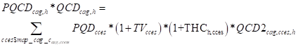
The Law of One Price (LOOP) must however be retained. Thus despite the demand for commodities by each household depending on c and h the prices paid (PQC) are only determined by the commodity c. However, since the mix of commodities in each aggregate commodity varies by household because the quantities of each natural commodity, the weights, are different for each household. Consequently, the aggregate prices (PQCD) are indexed on both the aggregate commodity, cag, and the household, h (P2). Two points deserve emphasis. The prices for aggregate commodities entering into the LES function cannot, by definition, be charged VAT (TV) since they have no real equivalent. But the value of the aggregate commodities must be defined so that they include any VAT paid on the natural commodities that make up the aggregate commodities. Secondly, the requirement for elasticity estimates is both increased and made empirically more difficult. The increase in empirical difficulty is that substitution elasticities are required for the components of the aggregate commodities; the income elasticities of demand are for aggregates, which is actually the situation encountered with standard implementations of LES functions.
The price of the natural commodities (PQC) is defined as the domestic price of the commodities (PQD) charged of the VAT (TV) and of the food aid tax (THS) (P3).
The price block is completed by two price indices that can be used for price normalisation. Equation (N1) is for the consumer price index (CPI), which is defined as a weighted sum of composite commodity prices (PQD) in the current period, where the weights are the shares of each commodity in total demand (comtotsh). The domestic producer price index (PPI) is defined (N2) by reference to the supply prices for domestically produced commodities (PD) with weights defined as shares of the value of domestic output for the domestic market (vddtotsh).
![]() (N1)
(N1)
![]() (N2)
(N2)
The supply prices of domestically produced commodities (X1) are determined by purchaser prices of those commodities on the domestic and international markets. Allowing for the possibility that the optimal output mix produced by an activity can vary according to the relative prices paid for the commodities produced by each activity means that the (weighted) average activity prices (PX) where the weights are quantities of each commodity produced by each activity (IOQXACQX). The determination of the optimal mixes of commodities produced by each activity are detailed below (X18). With CES technology the output by an activity, (QX) is determined by the aggregate quantities of factors used at the top level of the nested production function (X2).
In this model, a flexible production process is adopted, with
all the possible levels as a CES or Leontief function. With CES technology (X4)
the quantities of aggregate factors (fag) is aggregated as CES by the
quantities of factors used at the level below, where ![]() is the share
parameter,
is the share
parameter, ![]() is the
substitution parameter and
is the
substitution parameter and ![]() is
the efficiency variable (X). The efficiency factors (ADFAGfag,a)
and the factor shares (
is
the efficiency variable (X). The efficiency factors (ADFAGfag,a)
and the factor shares (![]() )
calibrated from the data and the elasticities of substitution, from which the
substitution parameters are derived (
)
calibrated from the data and the elasticities of substitution, from which the
substitution parameters are derived (![]() ),
are exogenously imposed. Note how the efficiency/shift factor is defined as a
variable and an adjustment mechanism is provided (X3), where adfagb is
the base values, dabfag is an absolute change in the base value, ADFAGADJ
and
),
are exogenously imposed. Note how the efficiency/shift factor is defined as a
variable and an adjustment mechanism is provided (X3), where adfagb is
the base values, dabfag is an absolute change in the base value, ADFAGADJ
and ![]() are
equiproportionate (multiplicative) adjustment factor. A shift parameter for
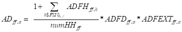
total efficiency (X4) is also calculated summing a shift parameter for factor
and activity specific efficiency (ADFD), a shift parameter for factor and
household specific efficiency (ADFH) affected by education and health
expenditure and the change in factor productivity due to extension services
affected by expenditure in extension services (See below). The matching first
order conditions (X5) define the wage rate for specific factors used by a
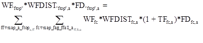
specific activity as the average wage rate for that factor (WFf) times a factor and activity
specific factor ‘efficiency’ parameter (WFDISTf,a). However the actual returns to a
factor must be adjusted to allow for taxes on factor use (TFf,a).
are
equiproportionate (multiplicative) adjustment factor. A shift parameter for
total efficiency (X4) is also calculated summing a shift parameter for factor
and activity specific efficiency (ADFD), a shift parameter for factor and
household specific efficiency (ADFH) affected by education and health
expenditure and the change in factor productivity due to extension services
affected by expenditure in extension services (See below). The matching first
order conditions (X5) define the wage rate for specific factors used by a
specific activity as the average wage rate for that factor (WFf) times a factor and activity
specific factor ‘efficiency’ parameter (WFDISTf,a). However the actual returns to a
factor must be adjusted to allow for taxes on factor use (TFf,a).
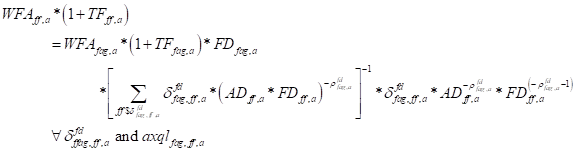
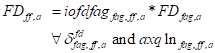
The flexible form of the production function allows the modeler to choose between a nest with Constant Elasticity of Substitution and Leontief technology on each level of the function. When the Leontief technology is chosen, the value of each aggregated nest is equal to the sum of the values of the factors composing that nest () while the quantity of the factor FD is defined as the product of the fixed (Leontief) input coefficients of demand for commodity c by activity a (iofdfag), multiplied by the quantity of the aggregated factor (FDfag) (X11). The choice of the aggregation function is controlled by the membership of the set aqx1 (CES), with the membership of aqx1n (Leontief) being the complement of aqx.
Each intermediate input (commodities) enter the flexible production factor as a production factor, X8 guarantees that the return of the factor WF is equal to the consumer price (PQD) at which intermediate inputs are evaluated. X9 calculates the sum of intermediate inputs per activity QINTa, while X10 calculates the quantity of each intermediate inputs in each activity. Equation X11 simply the previous equations by calculating the return to each factors as the wage times the distortion factor. X12 calculates the value added of each activity by summing the values of all natural factors employed.
![]() (X1)
(X1)
 (X2)
(X2)
![]() (X3)
(X3)
 (X4)
(X4)
 (X5)
(X5)
 (X6)
(X6)
 (X7)
(X7)
 (X8)
(X8)
![]() (X9)
(X9)
![]() (X10)
(X10)
![]() (X10b)
(X10b)
![]() (X10b)
(X10b)
![]() (X11)
(X11)
![]() (X11b)
(X11b)
![]() (X12)
(X12)
 (X13)
(X13)
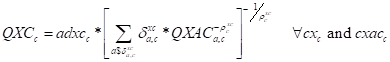
The composite supplies of each commodity (QXC) are
aggregates of the commodity outputs by each activity (QXAC). The default
assumption is that when a commodity is produced by multiple activities it is
differentiated by reference to the activity that produces the commodity; this
is achieved by defining total production of a commodity as a CES aggregate of
the quantities produced by each activity (X15). This provides a
practical/modelling solution for two typical situations; first, where there are
quality differences between two commodities that are notionally the same, e.g.,
modern digital vv disposable cameras, and second, where the mix of commodities
within an aggregate differ between activities, e.g., a cereal grain aggregate
made up of wheat and maize (corn) where different activities produce wheat and
maize in different ratios. This assumption of imperfect substitution is
implemented by a CES aggregator function with ![]() as the shift
parameter,
as the shift
parameter, ![]() as the share
parameter and
as the share
parameter and ![]() as the
elasticity parameter.
as the
elasticity parameter.
The matching first order condition for the optimal combination of commodity outputs is therefore given by (X16), where PXAC are the prices of each commodity produced by each activity. Note how, as with the case of the value added production function two formulations are given for the first-order conditions and the second version is the default version used in the model. Further note that the efficiency/shift factor is in this case declared as a parameter; this reflects the expectation that there will be no endogenously determined changes in these shift factors.
However, there are circumstances where perfect substitution may be a more appropriate assumption given the characteristics of either or both of the activity and commodity accounts. Thus an alternative specification for commodity aggregation is proved where commodities produced by different activities are modeled as perfect substitutes, (X17), and the matching price condition is therefore requires that PXAC is equal to PXC for relevant commodity activity combinations (X18). The choice of aggregation function is controlled by the membership of the set cxac, with the membership of cxacn being the complement of cxac.
Finally, it is necessary to determine the quantities of each commodity produced by each activity. There are two basic assumptions included in the model: first that secondary commodities are produced with pure by-product technologies, i.e., in a fixed ratio to the principle product, and second that activities can adjust their output mix in response to changes in the prices of the commodities they produce. The function for by-product assumption is that fixed shares of products (IOQXACQX) are produced by each activity according to its level of total output (QX); although the shares are defined as variable the user determines which rows of the matrix IOQXACQX are fixed when configuring the model by defining membership of the set acet (X19). In order to implement the alternative assumption, it is only necessary to specify the first order condition for a CET function; this is reported in equation (X20). However, it is also now necessary to include a market clearing condition for production; this is reported in the market clearing section below (see equation C2).
 (X14)
(X14)
 (X15)
(X15)
![]() (X15b)
(X15b)
![]() (X16)
(X16)
![]() (X17)
(X17)
![]() (X18)
(X18)
 (X19)
(X19)
![]() (X19b)
(X19b)
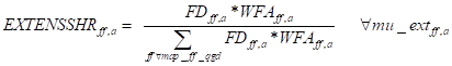
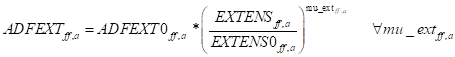
The provision of extension services by the government has the effect to increase productivity of a series of factors affected by this provision. The share of extension services (Ext2) benefiting to each factor is multiplied by the public expenditure in extension to calculate the expenditure in extension by factor (Ext1). The change in factor productivity due to extension services is calculated by the change in the expenditure in extension versus the initial level with a given elasticity mu_ext (Ext 3).
![]() (Ext
1)
(Ext
1)
![]() (Ext
1b)
(Ext
1b)
 (Ext
2)
(Ext
2)
![]() (Ext
2b)
(Ext
2b)
 (Ext 3)
![]() (Ext
3b)
(Ext
3b)
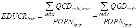
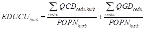
The provision of education and health services by the government has the effect to increase productivity of a series of factors affected by this provision. The per capita expenditure of education is the sum of private and public expenditure in education in rural and urban areas dived by population (Edu 1 and Edu2). The per capita expenditure of health is the sum of private and public expenditure in education in rural and urban areas divided by population (Edu4).
The change in factor productivity due to education and health services is calculated by the change in the expenditure in education and health versus the initial level with a given elasticity mu_ed and mu_he.
 (Edu1)
 (Edu2)
![]() (Edu3)
(Edu3)
 (Edu4)
 (Edu5)
There are two sources of income for factors. First there are payments to factor accounts for services supplied to activities, i.e., domestic value added, and second there are payments to domestic factors that are used overseas, the value of these are assumed fixed in terms of the foreign currency. Factor incomes (YF) are therefore defined as the sum of all income to the factors across all activities (F1)
![]() (F1)
(F1)
![]() (F2)
(F2)
 (F3)
(F3)
 (F4)
(F4)
![]() (F4b)
(F4b)
![]() (F5)
(F5)
![]() (F5b)
(F5b)
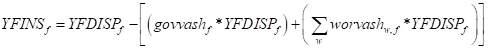
Before distributing factor incomes to the institutions that supply factor services allowance is made for depreciation rates (deprec) and factor (income) taxes (TYF) so that factor income for distribution (YFDISP) is defined (F2).
The endogenous determination of factor incomes requires the definition of variables that control that distribution. The key assumption is that the shares of factor income (FSISH) distributed to institutions (insw) are defined by the shares of factor ownership (FSI), which is implemented in (F3). For coding convenience the values of factor incomes distributed to each institution (INSVA) are calculated explicitly (F4); this reduces the code needed later although it increases the number of variables in the model.
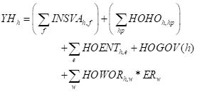
Households receive income from a variety of sources (H1). Factor incomes are distributed to households in proportion to their ownership of factors (INSVAh,f), plus inter household transfers (HOHO), distributed payments/dividends from incorporated enterprises (HOENT) and real transfers from government (HOGOV) and transfers from the rest of the world (HOWOR) converted into domestic currency units.
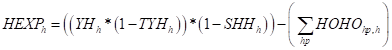
Inter household transfers (HOHO) are defined (H2) as a fixed proportions of household income (YH) after payment of direct taxes and savings. Real government transfers to households (HOGOV) are adjustable using multiplicative and additive scaling factors (H4)
Household consumption expenditure (HEXP) is defined as household income after tax income less savings and transfers to other households (H3).
 (H1)
(H1)
![]() (H2)
(H2)
![]() (H2b)
(H2b)
 (H3)
(H3)
![]() (H4)
(H4)
![]() (H5)
(H5)
![]() (H5b)
(H5b)
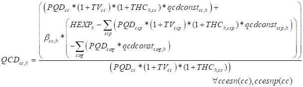
Households are then assumed to maximise utility subject to nested CES and Stone-Geary (aka LES) utility functions. In a Stone-Geary utility function household consumption demand consists of two components; ‘subsistence’ demand (qcdconst) and ‘discretionary’ demand, and the equation must therefore capture both elements. This is written as two equation, (H4) and (H5), where the first encompasses the natural commodities that are independent arguments in the utility function and the second encompasses the aggregate commodities. Discretionary demand is then defined as the marginal budget shares (beta) spent on each commodity out of ‘uncommitted’ income, i.e., household consumption expenditure less total expenditure on ‘subsistence’ demand of BOTH natural and aggregate commodities. In this system of nested utility functions, the commodities in the LES utility function are (typically) defined as ‘broad’ commodity groups, e.g., food, clothing, utilities, etc., that are aggregates of ‘natural’ commodities or ‘natural’ commodities that are deemed sufficiently distinctive as to justify the assumption that they are characterised by having a distinct level of ‘subsistence’ demand. The set cles(cc) is therefore defined to encompass all commodities, natural or aggregated, that enter into the LES utility functions, and the LES function is calibrated accordingly. If the user wants to assume Cobb-Douglas utility functions, at the top level, for one or more households this can be achieved by setting the Frisch parameters equal to minus one and all the income elasticities of demand equal to one (the model code includes documentation of the calibration steps). This is typically only the case for relatively rich households where the operation of the utility function will not reduce demand below a level consistent with subsistence demand.
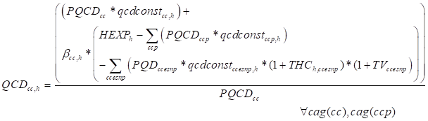
The second level of the utility functions is defined with CES preferences. The quantities of the aggregated commodity groups that are demanded by each household (QCDcag,,h) are defined in the top level (LES) utility function and therefore only the first order conditions are required to determine the optimum combinations of natural commodities. This is presented as a standard FOC for a CES function which has been calibrated for shift, share and elasticity parameters based on the initial data and the, exogenous imposed, substitution elasticities that are aggregate commodity and household specific.
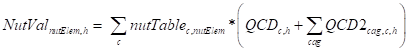
If a nutritional table exists and can be mapped to the commodities of the SAM, the model calculates the values of nutritional elements consumed by each household (H9).
 (H6)
(H6)
![]() (H6b)
(H6b)
 (H7)
(H7)
 (H8)
(H8)
![]() (H8b)
(H8b)
 (H9)
(H9)
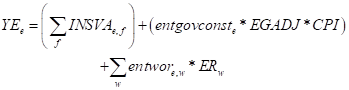
Similarly, income to enterprises (EN1) comes from the share of distributed factor incomes accruing to enterprises (INSVAe,f) and real transfers from government (entgovconst) that are adjustable using a scaling factor (EGADJ) and the rest of the world (entwor) converted in the domestic currency units.
 (EN1)
(EN1)
![]() (EN2)
(EN2)
 (EN3)
(EN3)
 (EN4)
(EN4)
![]() (EN5)
(EN5)
The consumption of commodities by enterprises (QED) is defined (EN2) in terms of fixed volumes (qedconst), which can be varied via the volume adjuster (QEDADJ), and associated with any given volume of enterprise final demand there is a level of expenditure (VED); this is defined by (EN5) and creates an option for the macroeconomic closure conditions that distribute absorption across domestic institutions (see below).
If QEDADJ is made flexible, then qedconst ensures that the quantities of commodities demanded are varied in fixed proportions; clearly this specification of demand is not a consequence of a defined set of behavioural relationships, as was the case for households, which reflects the difficulties inherent to defining utility functions for non-household institutions. If VED is fixed then the volume of consumption by enterprises (QED) must be allowed to vary, via the variable QENTDADJ.
The incomes to households from enterprises, which are assumed to consist primarily of distributed profits/dividends, are defined by (EN3), where hoentsh are defined as fixed shares of enterprise income after payments of direct/income taxes, savings and consumption expenditure. Similarly the income to government from enterprises, which is assumed to consist primarily of distributed profits/dividends on government owned enterprises, is defined by (EN4), where goventsh is defined as a fixed share of enterprise income after payments of direct/income taxes, savings and consumption expenditure.
All tax rates are variables in this model. The tax rates in the base solution are defined as parameters, e.g., tmbc are the import duties by commodity c in the base solution, and the equations then allow for varying the tax rates in 4 different ways. For each tax instrument there are four methods that allow adjustments to the tax rates; two of the methods use variables that can be solved for optimum values in the model according to the choice of closure rule and two methods allow for deterministic adjustments to the structure of the tax rates. The operation of this method is discussed in detail only for the equations for import duties while the other equations are simply reported.
Import duty tax rates are defined by (GT1), where tmbc is the vector of import duties in the base solution, dabtmc is a vector of absolute changes in the vector of import duties, TMADJ is a variable whose initial value is ONE, DTM is a variable whose initial value is ZERO and tm01c is a vector of zeros and non zeros. In the base solution the values of tm01c and dabtmc are all ZERO and TMADJ and DTM are fixed as their initial values – a closure rule decision –then the applied import duties are those from the base solution. Now the different methods of adjustment can be considered in turn
1. If TMADJ is made a variable, which requires the fixing of another variable, and all other initial conditions hold then the solution value for TMADJ yields the optimum equiproportionate change in the import duty rates necessary to satisfy model constraints, e.g., if TMADJ equals 1.1 then all import duties are increased by 10%.
2. If any element of dabtm is non zero and all the other initial conditions hold, then an absolute change in the initial import duty for the relevant commodity can be imposed using dabtm, e.g., if tmb for one element of c is 0.1 (a 10% import duty) and dabtm for that element is 0.05, then the applied import duty is 0.15 (15%).
3. If TMADJ is a variable, any elements of dabtm are non zero and all other initial conditions hold then the solution value for TMADJ yields the optimum equiproportionate change in the applied import duty rates.
4. If DTM is made a variable, which requires the fixing of another variable, AND at least one element of tm01 is NOT equal to ZERO then the subset of elements of c identified by tm01 are allowed to (additively) increase by an equiproportionate amount determined by the solution value for DTM times the values of tm01. Note how in this case it is necessary to both ‘free’ a variable and give values to a parameter for a solution to emerge.
This combination of alternative adjustment methods covers a range of common tax rate adjustment used in many applied applications while being flexible and easy to use.
Export tax rates are defined by (GT2), where tmec is the vector of export duties in the base solution, dabtec is a vector of absolute changes in the vector of export duties, TEADJ is a variable whose initial value is ONE, DTE is a variable whose initial value is ZERO and te01c is a vector of zeros and non zeros. Sales tax rates are defined by (GT3), where tmsc is the vector of sales tax rates in the base solution, dabtsc is a vector of absolute changes in the vector of sales taxes, TSADJ is a variable whose initial value is ONE, DTS is a variable whose initial value is ZERO and ts01c is a vector of zeros and non zeros. And excise tax rates are defined by (GT6), where texbc is the vector of excise tax rates in the base solution, dabtexc is a vector of absolute changes in the vector of import duties, TEXADJ is a variable whose initial value is ONE, DTEX is a variable whose initial value is ZERO and tex01c is a vector of zeros and non zeros. The model also allows for specific, quantity rather than value based, taxes on commodities (TQS) in equation GT4, and value added taxes (TV) in equation GT5.
![]() (GT1)
(GT1)
![]() (GT2)
(GT2)
![]() (GT3)
(GT3)
![]() (GT4)
(GT4)
![]() (GT4b)
(GT4b)
![]() (GT5)
(GT5)
![]() (GT6)
(GT6)
![]() (GT7)
(GT7)
![]() (GT7b)
(GT7b)
![]() (GT8)
(GT8)
![]() (GT9)
(GT9)
![]() (GT10)
(GT10)
![]() (GT11)
(GT11)
Indirect tax rates on production are defined by (GT7), where txbc is the vector of production taxes in the base solution, dabtxc is a vector of absolute changes in the vector of production taxes, TXADJ is a variable whose initial value is ONE, DTX is a variable whose initial value is ZERO and tx01c is a vector of zeros and non zeros. Taxes on factor use by each factor and activity are defined by (GT8), where tfbf,a is the matrix of factor use tax rates in the base solution, dabtff,a is a matrix of absolute changes in the matrix of factor use taxes, TFADJ is a variable whose initial value is ONE, DTFM is a variable whose initial value is ZERO and tf01f,a is a matrix of zeros and non zeros.
Factor income tax rates are defined by (GT9), where tyfbf is the vector of factor income taxes in the base solution, dabtyyf is a vector of absolute changes in the vector of factor income taxes, TYFADJ is a variable whose initial value is ONE, DTYF is a variable whose initial value is ZERO and tyf01f is a vector of zeros and non zeros. Household income tax rates are defined by (GT10), where tyhbh is the vector of household income tax rates in the base solution, dabtyhh is a vector of absolute changes in the vector of income tax rates, TYFADJ is a variable whose initial value is ONE, DTYF is a variable whose initial value is ZERO and tyh01c is a vector of zeros and non zeros. And finally, enterprise income tax rates are defined by (GT11), where tyebe is the vector of enterprise income tax rates in the base solution, dabtyee is a vector of absolute changes in the income tax rates, TYEADJ is a variable whose initial value is ONE, DTYE is a variable whose initial value is ZERO and tye01e is a vector of zeros and non zeros.
Although it is not necessary to keep the tax revenue equations separate from other equations, e.g., they can be embedded into the equation for government income (YG), it does aid clarity and assist with implementing fiscal policy simulations. For this model there are eight tax revenue equations. The patterns of tax rates are controlled by the tax rate variable equations. In all cases the tax rates can be negative indicating a ‘transfer’ from the government.
There are four tax instruments that are dependent upon expenditure on commodities, with each expressed as an ad valorem tax rate. Tariff revenue (MTAX) is defined (GR1) as the sum of the product of tariff rates (TM) and the value of expenditure on imports at world prices, the revenue from export duties (ETAX) is defined (GR2) as the sum of the product of export duty rates (TE) and the value of expenditure on exports at world prices, the sale tax revenues (STAX) are defined (GR3) as the sum of the product of sales tax rates (TS) and the value of domestic expenditure on commodities, and excise tax revenues (EXTAX) are defined (GR5) as the sum of the product of excise tax rates (TEX) and the value of domestic expenditure on commodities. The model also allows for specific, quantity rather than value based, taxes (GR4) on commodities (QSTAX) where the base for the tax is the quantity of the commodity rather than value. There is also provision for value added tax (GR5) where as opposed to other taxes and commodities demanded domestically the tax is only paid on final demand by households.
![]() (GR1)
(GR1)
![]() (GR2)
(GR2)
![]() (GR3)
(GR3)
![]() (GR4)
(GR4)
 (GR5)
(GR5)
![]() (GR6)
(GR6)
![]() (GR7)
(GR7)
![]() (GR8)
(GR8)
![]() (GR9)
(GR9)
![]() (GR10)
(GR10)
There is a single tax on production (ITAX). As with other taxes this is defined (GR7) as the sum of the product of indirect tax rates (TX) and the value of output by each activity evaluated in terms of the activity prices (PX). In addition activities can pay taxes based on the value of employed factors – factor use taxes (FTAX). The revenue from these taxes is defined sum of the product of factor income tax rates and the value of the factor services employed by each activity for each factor; the sum is over both activities and factors. These two taxes are the instruments most likely to yield negative revenues through the existence of production and/or factor use subsidies.
Income taxes are collected on both factors and domestic institutions. The income tax on factors (FYTAX) is defined (GR9) as the product of factor tax rates (TYF) and factor incomes for all factors, while those on institutions (DTAX) are defined (GR10) as the sum of the product of household income tax rates (TYH) and household incomes plus the product of the direct tax rate for enterprises (TYE) and enterprise income.
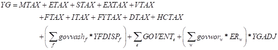
The sources of income to the government account (G1) are more complex than for other institutions. Income accrues from 9 tax instruments; tariff revenues (MTAX), export duties (ETAX), value added taxes (VTAX), (general) sales taxes (STAX), excise taxes (EXTAX), production taxes (ITAX), factor use taxes (FTAX), factor income taxes (FYTAX) and direct income taxes (DTAX), which are defined in the tax equation block above. In addition the government can receive income from its ownership of factors (INSVA), distributed payments/dividends from incorporated enterprises (GOVENT) and transfers from abroad (govwor) converted in the domestic currency units. It would be relatively easy to subsume the tax revenue equations into the equation for government income, but they are kept separate to facilitate the implementation of fiscal policy experiments. Ultimately however the choice is a matter of personal preference.
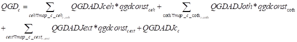
The demand for commodities by the government for consumption (QGD) is defined (G2) in terms of fixed proportions (qgdconst) that can be varied with a scaling adjuster (QGDADJ), and associated with any given volume of government final demand there is a level/value of expenditure (VGD) defined by (G3); this creates an option for the macroeconomic closure conditions that distribute absorption across domestic institutions (see below).
 (G1)
(G1)
 (G2)
(G2)
![]() (G3)
(G3)
 (G4)
(G4)
![]() (G5)
(G5)
Hence, total government expenditure (EG) can be defined (G4) as equal to the sum of expenditure by government on consumption demand at current prices, plus real transfers to households (hogovconst) that can be adjusted using a (multiplicative) scaling factor (HGADJ) and real transfers to enterprises (entgovconst) that can also be adjusted by a (multiplicative) scaling factor (EGADJ).
As with enterprises there are difficulties inherent to defining utility functions for a government. Changing QGDADJ, either exogenously or endogenously, by allowing it to be a variable in the closure conditions, provides a means of changing the behavioural assumption with respect to the ‘volume’ of commodity demand by the government. If the value of government final demand (VGD) is fixed then government expenditure is fixed and hence the volume of consumption by government (QGD) must be allowed to vary, via the QGDADJ variable. If it is deemed appropriate to modify the patterns of commodity demand by the government then the components of qgdconst must be changed.
Combining total government consumption expenditure and spending on government-related investment types iGovAgr, the total government budget (GBUDG) is defined in equation (G5).
The government agriculture related income and expenditure values are reported through a set of agricultural budget variables. The recurrent agricultural budget (G6) is defined as total government spending on agricultural commodities. Given that the base specification implies fixing government consumption (QGD), the recurrent budget changes follow the changes in agricultural commodity prices (PQD). Similarly to equation (I6), the investment budget across the different agricultural investment types iGovAgr (G7) is determined by a corresponding investment share (INVSH_I) in the total investment expenditure (INVEST). The input subsidy (AgBuInpSub) and the output subsidy (AgBuOutSub) budgets across agricultural activities aGovAgr are defined in equations (G8) and (G9) respectively. Equation (G10) determines the commodity price subsidies destined for households (AgBuComSub) which takes into account possible subsidies applied to both household demand variables, QCD and QCD2. Agricultural income subsidies are defined in equation (G11) as the value of government transfers to rural households. Equations (G12) – (G17) calculate the totals of the agricultural budget variables. The total agricultural budget is then determined as the sum of these budget variables (G18). Finally, the share of this total agricultural budget in the total government budget AgBuTOTShr is determined in equation (G19).
![]() (G6)
(G6)
![]() (G7)
(G7)
![]() (G8)
(G8)
![]() (G9)
(G9)
![]() (G10)
(G10)
![]() (G11)
(G11)
![]() (G12)
(G12)
![]() (G13)
(G13)
![]() (G14)
(G14)
![]() (G15)
(G15)
![]() (G16)
(G16)
![]() (G17)
(G17)
![]() (G17)
(G17)
![]() (G19)
(G19)
The savings rates for households (SHH in I1) and enterprises (SEN in I2) are defined as variables using the same adjustment mechanisms used for tax rates; shhbh and senbe are the savings rates in the base solution, dabshhh and dabsene are absolute changes in the base rates, SHADJ and SEADJ are multiplicative adjustment factors, DSHH and DSEN are additive adjustment factors and shh01h and sen01e are vectors of zeros and non zeros that scale the additive adjustment factors. However, unlike the tax rate equations, each of the savings rates equations has two additional adjustment factors – SADJ and DS. These serve to allow the user to vary the savings rates for households and enterprises in tandem; this is useful when the macroeconomic closure conditions require increases in savings by domestic institutions and it is not deemed appropriate to force all the adjustment on a single institution or group of institutions.
Total savings in the economy are defined (I3) as shares (SHH) of households’ after tax income, where direct taxes (TYH) have first call on household income, plus the allowances for depreciation at fixed rates (deprec) out of factor income, the savings of enterprise savings at fixed rates (SEN) out of after tax income, the government budget deficit/surplus (KAPGOV) and the current account ‘deficit’ (CAPWOR). The last two terms of I3 – KAPGOV and CAPWOR - are defined below by equations in the market clearing block.
![]() (I1)
(I1)
![]() (I2)
(I2)
 (I3)
(I3)
![]() (I4)
(I4)
![]() (I4b)
(I4b)
![]() (I5)
(I5)
![]() (I6)
(I6)
![]() (I7)
(I7)
The presence of multiple types of capital goods implies the existence of different patterns of investment expenditures each corresponding to one type of capital good, where the set i defines the investment patterns and each member of i is uniquely paired with a member of the set k (capital factors). In essence, this implies that each capital good has a unique cost of production (a form of ‘production function’) defined by the quantities of each commodity required to produce a given quantity of the capital good. If the functional form for the ‘production functions’ are assumed to be Leontief it is possible to derive input-output coefficients that define the quantities of each input/commodity required to produce a unit of each capital good (ioqinvdc,i). Then the demand for each commodity used to produce investment goods (QINVDc,i) as the product of the quantity/volume of each capital good (QINVi) and the respective coefficients (ioqinvdc,i); these relationships are defined in I4 and I5.
The demand for commodities for investment purposes therefore depends on the ‘technologies’ and the volumes of capital goods required. However, comparative static and recursive dynamic CGE models do not have endogenously determined investment functions that serve to define the quantities of capital goods produced. A simple, and very commonly used, dichotomy is to assume that the demand for capital goods is determined by either the amount of available investable funds – so-called savings driven assumption - or exogenously – so-called investment driven or Keynesian assumption. Assume, for purposes of exposition only, that an investment driven assumption of exogenous determination is appropriate, i.e., QINVi is fixed exogenously.
To implement the investment driven assumption, the parameters qinvbi are fixed, at the exogenously determined levels, and the scaling variable IADJ is fixed equal to one (I5); and hence the demand for each commodity for investment purposes are determined from I4. Given the demand for each commodity and the prices for each commodity (PQDc) the value of investment expenditures to produce each capital good i (INVEST*INVSH_Ii) is the product of prices and quantities (I6). The total value of all investments (INVEST) is then defined as the summation of the expenditures on each capital good (I7), and market clearing for investable funds is ensure by the equality of total savings (TOTSAV) and investment (see C20 below).
If a savings driven assumption is adopted, then the value of INVEST is determined by total savings (TOTSAV) and the parameters qinvbi determine the ratio of capital goods produced with the scaling variable IADJ providing (multiplicative) equiproportionate changes in the volumes of each capital good. The scaling variable IADJ adjusts the volumes of capital goods produced so that the expenditures on each capital good (INVEST*INVSH_Ii ) exhaust the available investable funds (INVEST); thus in such a setting I7 operates as a market clearing equation.
The members of the set i include the agent that gathers together investable funds from savings by domestic and foreign agents (‘i_s’) and distributes those funds across different investment activities. One such investment activity is stock changes (‘dstoc’); thus stock changes can be included within this formulation.
In a comparative static context, the specification of different patterns of investment expenditures is relevant if and only if the analyst has information that indicates that the average pattern of investment expenditures will change due to the simulation. If the relative volumes of investment in capital goods is invariant, then the system operates as if there is a single investment account, i.e., the system de facto collapses back to the ‘standard’ approach in the STAGE family of models.
The economy also employs foreign owned factors whose services must be recompensed. It is assumed that these services receive proportions of the factor incomes available for distribution, (W1).
![]() (W1)
(W1)
The description immediately below refers to a default set of closure rules/market clearing conditions for this model; a subsequent section explores alternative closure rules//market clearing configurations available with this model.
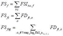
The factor market is cleared by equating factor demands (FD) plus unemployment (UNEMP) and factor supplies by institutions (FSI) for all factors (C1), and the supplies of each factor (FS) equal factor supplies by institutions (FSI) for all factors (C2).
The unemployment is calculated following a typical MCP regime switching definition. Unemployment is greater or equal to zero (C4). When unemployment is equal to zero, the wage rate of unemployed sector is fixed and the change in factor supply clears the market. When unemployment is equal to zero, the wage becomes endogenous and clear the market while the factor supply is fixed (fully employed). The unemployment rate is calculated as the rate between unemployed and supply of each factor (C5).
Importantly, the factors (labour) used by institutions to produce leisure can only be supplied by the specific institution. Thus the factor quantities supplied by each institution for the production of leisure (FSIL) must be defined so as to be activity, and its paired RHG, and factor specific This is defined in equation C5 where the mapping (map_hh_alei) pairs leisure activities (alei) with RHGs (hh). Then the market clearing condition for the factor supplies by institution (FSI) and the demand for factors by non-leisure activities (FD) and leisure activities (FSIL) are determined as residuals.
![]() (C1)
(C1)
 (C2)
(C2)
![]() (C2b)
(C2b)
![]() (C3)
(C3)
![]() (C4)
(C4)
![]() (C5)
(C5)
There is however no reason to suppose that the proportionate changes in the amount of labour time devoted to leisure and non-leisure activities will be identical across households. Even if the elasticities controlling the operation of the RHGs utility functions are the same there are differences in the levels of household incomes and preferences, i.e., there will be differences in the shift and share parameters of the utility functions. Thus the presence of a labour-leisure trade-off means that the labour/factor supplies by institution (FSI) will be endogenously determined variables and hence the functional distribution of income can change.
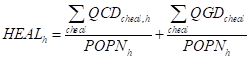
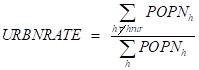
Changes in population influence the supply of labour factors (see Factor Mobility section below) and are function of the evolution of birth and death rates within each RHG. Both these demographic variables are endogenous in the model. Birth rates are determined in (P1) as a function of (EDUC) education spending by households and government on a per capita basis (P9). The inclusion of (EDUC) as a denominator together with specifying a positive elasticity of ‘birthrate to education spending’ imply that birth rates reduce with an increase in education spending. Similarly, in (P2) death rates are function of (HEAL) healthcare spending per capita by households and government combined (P10)– a higher spending from base period level (HEAL0) leads to a decrease in death rates. Next, total death and birth headcounts are calculated in (P3) and (P4) by factoring in total population for each RHG. Population change is then calculated as the difference between total births and total deaths (P5). Finally, population numbers (POPN) are updated from base period values (POPN_A) in (P7). To ensure consistency of between the changes in population and the factor supply of each RHG, total labour supply is equalised to the updated population count (P6). The country urbanisation rate is also updated to reflect changes in urban and rural population counts in (P8).
 P1
P1
 P2
P2
![]() P3
P3
![]() P4
P4
![]() P5
P5
![]() P6
P6
![]() P7
P7
 (P8)
(P8)
 (P9)
(P9)
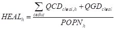 (P10)
(P10)
A typical approach to modelling representative household groups (RHG), one of the groups that make up institutions, is to assume that households are rigidly segmented and that each RHG receives a fixed share of factor incomes generated domestically and received from abroad. The first part of the assumption requires that households are not allowed to migrate, e.g., rural-urban migration is precluded, while the second part carries the implicit presumption that any changes in factor supplies by RHGs changes the supply of each factor by each RHG equiproportionately. Neither of these assumptions is necessarily an accurate reflection of reality and, at the same time, imposes restrictions that require households to NOT change behaviours in response to economic signals. This model allows RHGs to relocate/migrate in response to changes in economic signals, e.g., changes in relative RHG incomes, and, when they do so, to transfer their factors from the RHG they leave to the RHG they join, i.e., modifying the factor supplies by households (FSI) and hence the functional distribution of income. The model is coded so that the functional distribution of income changes as RHGs migrate; the logic of the code is the same as that used to allow factor mobility functions (see below).
The inclusion of the assumption of household migration across types of household relaxes the restrictive assumption of rigid segmentation of RHGs. The behavioural assumption is that the incentives for a RHG to migrate in the model are changes in the relative returns to different RHGs, i.e., only economic incentives are embodied within the behavioural assumption. Thus if RHGs in one segment experiences a RELATIVE increase in income to the RHGs in all other segments there will be incentives for households to relocate/migrate to the RHG that receives an increase in RELATIVE income: relative incomes (YMIGR) are defined in (Mig1). Relative income changes are then calculated in the income per capita migration driver HMIGDRV using the relative income in the base period (YMIGRA) as reference (Mig4).
It is important to note that the user needs to specify the set (inswmig) that defines the pairs of RHGs between which households can migrate. This is defined as a dynamic set to which pairs of RHGs are assigned if a corresponding migration elasticity etam is specified.
 (Mig1)
 (Mig2)
 (Mig3)
![]() (Mig3b)
(Mig3b)
![]() (Mig4)
(Mig4)
![]() (Mig4b)
(Mig4b)
 (Mig5)
![]() (Mig6)
(Mig6)
![]() (Mig7)
(Mig7)
 (Mig8)
A typical approach to factor supply and demand is that factors are rigidly segmented so that the total available supply of a factor is fixed, either at the current level of total demand, i.e., full employment, or at some level that is greater than the current level of total demand so as to allow for unemployment of that type of factor. This presumption of rigid segmentation is restrictive and as such does not allow for the possibility that labour can transition, to a greater or lesser extent, between the segments in response to changes in the factor market with or without job specific training. This can be especially problematic when labour types are classified by occupational categories, e.g., clerks, shop workers, agricultural workers, etc. For instance, tractor operators, in agriculture, may readily transition into JCB operators, in construction, but if they are classified as agricultural workers and construction workers respectively, many model close off this transition option. Moreover, a common option of classifying labour by levels of skill, e.g., skilled, semi-skilled and unskilled, involves the implicit assumption that all labour of a specific type receives the same average wage rate when within each type of labour there is likely to be a range of wage rates about the average. Thus, it may be that lower paid skilled workers may be willing to take employment as semi-skilled workers if average wage rates for skilled workers decline relative to those of semi-skilled workers.
These differences in average wage rates are reflected in the fact that workers of the same notional type are typically paid at different wage rates according to the activity in which they are employed. This is evident in any CGE model for which there are data for both the transactions values and quantities of labour employed by different activities; in this model these differences are reported by the values of WFDISTf,a. Where such data are available it is not uncommon to find that skilled agricultural workers are paid less than semi-skilled manufacturing workers. Such an observation implies, within the logic of CGE models and the labour classification scheme, that the labour market is not operating efficiently. Such an observation is typically, if at all, justified by some combination of assuming that there are non-rewarded preferences that explain the differences in average wages and/or that the differences are entirely due to activity specific attributes, i.e., the maintained assumption is that the labour classification scheme encompasses all differences in characteristics of the labour types. But it does mean that any reallocations of labour in simulations can and, typically, does result in changes in the average productivity of labour, which is equivalent to changing the factor endowments in the model.
The inclusion of the assumption of factor mobility across types of labour relaxes this restrictive assumption by assuming that types of factors can transition into other, specified, types in response to changes in the relative wages (WMIGR). Therefore, similar to the income per capita driver definition from above, the model includes a relative wage migration driver. A relative wage (WMIGR) is calculated in equation (Mig2) for every factor pair for which a transition is possible. This relative wage is calculated as the ratio of average wages of the factor pair, accounting for the unemployment rates of the two factors. Finally, the relative wage migration driver for each factor pair is calculated as the ratio between the relative wage (WMIGR) and the reference relative wage in the base period (WMIGRA). Similar to the household pairs inswmig, the factor pairs in the set (fmig) comprising the factors for which migration can change supply values are validated as long as the etam migration elasticity is defined. In case (fmig) is not defined for a pair of factors, than the wage migration factor is fixed to the base period value (FMIGDRV0), normally set at 0 (Mig3b).
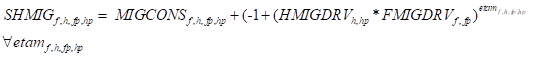
The compounded effect on the two migration drivers is introduced when calculating the share of population migrating (SHMIG). Equation (Mig5) calculates this share and allows for the specification of a constant part (MIGCONS) in case other exogenous drivers of migration need to be factored in. The variable part of the equation includes the net effect of the income per capita (HMIGDRV) and the wage (FMIGDRV) drivers, controlled by the migration elasticity etam which can be specified across all household and factor pairs. The factors that are migrating from institution hp to h and from factor fp to f are then a function of the share of the population in migrating and the base period factor supply fsia by institution hp of factor fp – equation (Mig6).
Total factor supply by each institution/RHG is the updated (Mig7) by taking into account changes in factor supply due to population growth (Mig 8) and the net effect of migration. The net effect takes into account both migrations of households and factors to the institution/RHG and out of the institution/RHG.
Connected to the household migration and labour mobility, the endogeneity of the functional distribution is ensured by the fact that the functional distribution of income depends upon the shares of factors supplied by different institutions (FSISH), which is a function of the supply of factors by institutions (FSI), which is defined in Eqn (C6). Since both of these are endogenous variables the functional distribution of income is endogenous.
Market clearing for the composite commodity markets requires that the supplies of the composite commodity (QQ) are equal to total of domestic demands for composite commodities, which consists of intermediate demand (QINTD), household (QCD and QCD2), enterprise (QED) and government (QGD) and investment (QINVD) final demands (C13). Note how the market clearing condition with respect to final demand by households has to be formulated so as to avoid double counting by ensuring that no aggregate commodities enter into the definition (RHS) of domestic demand. Since the markets for domestically produced commodities are also cleared (X16) this ensures a full clearing of all commodity markets. Similarly, it is necessary to ensure clearing of the production of differentiated commodities by activities when activities can adjust their output mixes in response to changes in relative commodity prices; this is done in equation (C12).
![]() (C12)
(C12)
 (C13)
(C13)
Making savings a residual for each account clears the two institutional accounts that are not cleared elsewhere – government and rest of the world. Thus the government account clears (C14) by defining government savings (KAPGOV) as the difference between government income and other expenditures, i.e., a residual. The rest of world account clears (C15) by defining the balance on the capital account (CAPWOR) as the difference between expenditure on imports, of commodities and factor services, and total income from the rest of the world, which includes export revenues and payments for factor services, transfers from the rest of the world to the household, enterprise and government accounts, i.e., it is a residual.
![]() (C14)
(C14)
 (C15)
(C15)
![]()
The total value of domestic final demand (VFDOMD) is defined (C16) as the sum of the expenditures on final demands by households and other domestic institutions (enterprises, government and investment). Note again that the value of final demand must exclude the demand for aggregate commodities to avoid double counting.
It is also useful to express the values of final demand by each non-household domestic institution as a proportion of the total value of domestic final demand; this allows the implementation of what has been called a ‘balanced macroeconomic closure’. Hence the share of the value of final demand by enterprises (C17) can be defined as a proportion of total final domestic demand, and similarly for government’s value share of final demand (C18)
and for investment’s value share of final demand (C19).
If the share variables (VEDSH, VGDSH and INVESTSH) are fixed then the quantity adjustment variables on the associated volumes of final demand by domestic non-household institutions (QEDADJ, QGDADJ and IADJ or S*ADJ) must be free to vary. On the other hand if the volume adjusters are fixed the associated share variables must be free so as to allow the value of final demand by ‘each’ institution to vary.
 (C16)
(C16)
![]() (C17)
(C17)
![]() (C18)
(C18)
![]() (C19)
(C19)
The final account to be cleared is the capital account. Total savings (TOTSAV), see I3 above, is defined within the model and hence there has been an implicit presumption in the description that the total value of investment (INVEST) is driven by the volume of savings. This is the market clearing condition imposed by (C20). But this market clearing condition includes another term, WALRAS, which is a slack variable that returns a zero value when the model is fully closed and all markets are cleared, and hence its inclusion provides a quick check on model specification.
![]() (C20)
(C20)
It is not necessary to include a variable in the model for GDP, since GDP is a simple summary ‘variable’ that can be calculated from the simulation results. However, it is convenient in some circumstances, e.g., while benchmarking a recursive dynamic model, to include GDP as a variable. In this model GDP is included as a variable that is calculated from the expenditure side, i.e., domestic absorption (valued a purchaser prices) plus exports (valued at basic prices) less imports (valued at basic prices), (C21).
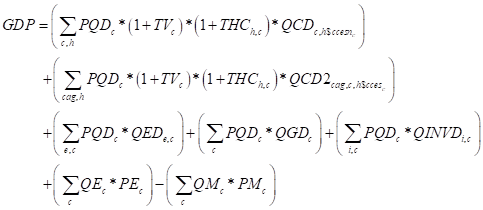 (C21)
(C21)
In mathematical programming terms the model closure conditions are, at their simplest, a matter of ensuring that the numbers of equations and variables are consistent. However economic theoretic dimensions of model closure rules are more complex, and, as would be expected in the context of an economic model, more important. The essence of model closure rules is that they define important and fundamental differences in perceptions of how an economic system operates (see Sen, 1963; Pyatt, 1987; Kilkenny and Robinson, 1990). The closure rules can be perceived as operating on two levels; on a general level whereby the closure rules relate to macroeconomic considerations, e.g., is investment expenditure determined by the volume of savings or exogenously, and on a specific level where the closure rules are used to capture particular features of an economic system, e.g., the degree of intersectoral capital mobility.
This model allows for a range of both general and specific closure rules. The discussion below provides details of the main options available with this formulation of the model by reference to the accounts to which the rules refer.
The closure of the rest of the world account can be achieved by fixing either the exchange rate variable (AC1a) or the balance on the current account (AC1b). Fixing the exchange rate is appropriate for countries with a fixed exchange rate regime whilst fixing the current account balance is appropriate for countries that face restrictions on the value of the current account balance, e.g., countries following structural adjustment programmes. It is a common practice to fix a variable at its initial level by using the associated parameter, i.e., ***0, but it is possible to fix the variable to any appropriate value.
The model is formulated with the world prices for traded commodities declared as variables, i.e., PWMc and PWEc. If a strong small country assumption is adopted, i.e., the country is assumed to be a price taker on all world commodity markets, and then all world prices will be fixed. When calibrating the model the world prices will be fixed at their initial levels, (AC1c), but this does not mean they cannot be changed as parts of experiments.
However, the model allows a relaxation of the strong small country assumption, such that the country may face a downward sloping demand curve for one or more of its export commodities. Hence the world prices of some commodities are determined by the interaction of demand and supply on the world market, i.e., they are variables. This is achieved by limiting the range of world export prices that are fixed to those for which there are no export demand function, (AC1d), by selecting membership of the set cedn.
![]() (AC1b)
(AC1b)
 (AC1c)
![]() (AC1d)
(AC1d)
To ensure that aggregate savings equal aggregate investment, the determinants of either savings or investment must be fixed. There are multiple ways of achieving this result. For instance this can be achieved by fixing either the saving rates for households or the volumes of commodity investment. This involves fixing either the savings rates adjusters (AC2a) or the investment volume adjuster (AC2c). Note that fixing the investment volume adjuster (AC2b) means that the value of investment expenditure might change due to changes in the prices of investment commodities (PQD). Note also that only one of the savings rate adjusters should be fixed; if SADJ is fixed the adjustment in such cases takes place through equiproportionate changes in the savings rates of households and enterprises, if SHADJ is fixed the adjustment in such cases takes place through equiproportionate changes in the savings rates of households, and if SEADJ is fixed the adjustment in such cases takes place through equiproportionate changes in the savings rates of enterprises. Alternatively savings rates can be adjusted through the additive adjustment factors (DS, DSHH, DSEN) with the same relationships between the savings rates of different classes of institutions (AC2b). Note that there are other sources of savings. The magnitudes of these other savings sources can also be changed through the closure rules (see below).
 (AC2a)
 (AC2b)
![]() (AC2c)
(AC2c)
![]() (AC2d)
(AC2d)
![]() (AC2e)
(AC2e)
Fixing savings, and thus deeming the economy to be savings-driven, could be considered a Neo-Classical approach. Closing the economy by fixing investment could be construed as making the model reflect the Keynesian investment-driven assumption for the operation of an economy.
The model includes a variable for the value of investment (INVEST), which can also be used to close the capital account (AC2d). If INVEST is fixed in an investment driven closure, then the model will need to adjust the savings rates to maintain equilibrium between the value of savings (TOTSAV) and the fixed value of investment. This can only be achieved by changes in the volumes of commodities demanded for investment (QINVD) or their prices (PQD). But the prices (PQD) depend on much more than investment, hence the main adjustment must take place through the volumes of commodities demanded, i.e., QINVD, and therefore the volume adjuster (IADJ) must be variable, as must the savings rate adjuster (SADJ).
Alternatively the share of investment expenditure in the total value of domestic final demand can be fixed, (AC2e), which means that the total value of investment is fixed by reference to the value of total final demand, but otherwise the adjustment mechanisms follow the same processes as for fixing INVEST equal to some level.
Fixing the volumes of commodities demand by enterprises, (AC3a), closes the enterprise account. Note that this rule allows the value of commodity expenditures by the enterprise account to vary, which ceteris paribus means that the value of savings by enterprises (CAPENT) and thus total savings (TOTSAV) vary. If the value of this adjuster is changed, but left fixed, this imposes equiproportionate changes on the volumes of commodities demanded.
![]() (AC3a)
(AC3a)
![]() (AC3b)
(AC3b)
![]() (AC3c)
(AC3c)
If QEDADJ is allowed to vary then another variable must be fixed; the most likely alternative is the value of consumption expenditures by enterprises (VED) (AC3b). This would impose adjustments through equiproportionate changes in the volumes of commodities demanded, and would feed through so that enterprise savings (CAPENT) reflecting directly the changes in the income of enterprises (YE). Alternatively the share of enterprise expenditure in the total value of domestic final demand can be fixed, (AC3c), which means that the total value of enterprise consumption expenditure (VED) is fixed by reference to the value of total final demand, but otherwise the adjustment mechanisms follow the same processes as for fixing VED equal to some level.
Finally the scaling factor for enterprise transfers to households (HEADJ) needs fixing (AC3d).
The closure rules for the government account are slightly more tricky because they are important components of the model that are used to investigate fiscal policy considerations. The base specification uses the assumption that government savings are a residual; when the determinants of government income and expenditure are ‘fixed’, government savings must be free to adjust.
Thus in the base specification all the tax rates (variables) are fixed by declaring the base tax rates as parameters and then fixing all the multiplicative and additive tax rate scaling factors (AC4a – AC4r).
![]() (AC4a)
(AC4a)
![]() (AC4b)
(AC4b)
![]() (AC4c)
(AC4c)
![]() (AC4d)
(AC4d)
![]() (AC4e)
(AC4e)
![]() (AC4f)
(AC4f)
![]() (AC4g)
(AC4g)
![]() (AC4h)
(AC4h)
![]() (AC4i)
(AC4i)
![]() (AC4j)
(AC4j)
![]() (AC4k)
(AC4k)
![]() (AC4l)
(AC4l)
![]() (AC4m)
(AC4m)
![]() (AC4n)
(AC4n)
![]() (AC4o)
(AC4o)
![]() (AC4p)
(AC4p)
![]() (AC4q)
(AC4q)
![]() (AC4r)
(AC4r)
![]() (AC4s)
(AC4s)
![]() (AC4t)
(AC4t)
![]() (AC4u)
(AC4u)
![]() (AC4v)
(AC4v)
![]() (AC4v)
(AC4v)
![]() (AC4v)
(AC4v)
![]() (AC4v)
(AC4v)
![]() (AC4v)
(AC4v)
![]() (AC4v)
(AC4v)
![]() (AC4v)
(AC4v)
![]() (AC4v)
(AC4v)
![]() (AC4v)
(AC4v)
![]() (AC4v)
(AC4v)
![]() (AC4v)
(AC4v)
Consequently changes in tax revenue to the government are consequences of changes in the other variables that enter into the tax income equations (GR1 to GR8). The two other sources of income to the government are controlled by parameters, govvash and govwor, and therefore are not a source of concern for model closure.
Also note that because there are equations for the revenues by each tax instrument (GR1 to GR8) it is straightforward to adjust the tax rates to achieve a given volume of revenue from each tax instrument; this type of arrangement is potentially useful in circumstances where is is argued/believed that binding constraints upon the revenue possibilities from specific tax instruments.
In the base specification government expenditure is controlled by fixing the volumes of commodity demand (QGD) through the government demand adjuster (QGDADJ) in (AC4s). Alternatively either the value of government consumption expenditure (VGD) can be fixed, (AC4t), or the share of government expenditure in the total value of domestic final demand (VGDSH) can be fixed, (AC4u). The scaling factor on the values of transfers to households and enterprises through the household (HGADJ) and enterprise (EGADJ) adjusters, (AC4v and AC4w) also need to be fixed.
![]() (AC4s)
(AC4s)
![]() (AC4v)
(AC4v)
![]() (AC4w)
(AC4w)
This specification ensures that all the parameters that the government can/does control are fixed and consequently that the only determinants of government income and expenditure that are free to vary are those that the government does not directly control. Hence the equilibrating condition is that government savings, the internal balance, is not fixed.
If however the model requires government savings to be fixed (AC4x), then either government income or expenditure must be free to adjust. Such a condition might reasonably be expected in many circumstances, e.g., the government might define an acceptable level of borrowing or such a condition might be imposed externally.
In its simplest form this can be achieved by allowing one of the previously fixed adjusters (AC4a to AC4w) to vary. Thus if the sales tax adjuster (TSADJ) is made variable then the sales tax rates will be varied equiproportionately so as to satisfy the internal balance condition. More complex experiments might result from the imposition of multiple conditions, e.g., a halving of import duty rates coupled with a reduction in government deficit, in which case the variables TMADJ and KAPGOV would also require resetting. But these conditions might create a model that is infeasible, e.g., due to insufficient flexibility through the sales tax mechanism, or unrealistically high rates of sales taxes. In such circumstances it may be necessary to allow adjustments in multiple tax adjusters. One method then would be to fix the tax adjusters to move in parallel with each other.
However, if the adjustments only take place through the tax rate scaling factors the relative tax rates will be fixed. To change relative tax rates it is necessary to change the relevant tax parameters. Typically such changes would be implemented in policy experiment files rather than within the closure section of the model.
The model specification allows for a choice of two price normalisation equations (AC5a and AC5b), the consumer price index (CPI) and a producer price index (PPI). A numéraire is needed to serve as a base since the model is homogenous of degree zero in prices and hence only defines relative prices.
![]() (AC5a)
(AC5a)
![]() (AC5b)
(AC5b)
The factor market closure rules are more difficult to implement than many of the other closure rules. Hence the discussion below proceeds in three stages; the first stage sets up a basic specification whereby all factors are deemed perfectly mobile, the second stage introduces a more general specification whereby factors can be made activity specific and allowance can be made for unemployed factors, while the third stage introduces the idea that factor market restrictions may arise from activity specific characteristics, rather than the factor inspired restrictions considered in the second stage.
This factor market closure requires that the total supply (FSI) of and total demand for factors (FD) equate (AC6a). The total supplies of each factor are determined exogenously and hence
defines the first set of factor market closure conditions. The demands for factor f by activity a and the wage rates for factors are determined endogenously. But the model specification includes the assumption that the wage rates for factors are averages, by allowing for the possibility that the payments to notionally identical factors might vary across activities through the variable that captures the ‘sectoral proportions for factor prices’. These proportions are assumed to be a consequence of the use made by activities of factors, rather than of the factors themselves, and are therefore assumed fixed, (AC6b). Finally while it may seem that factor prices must be limited to positive values the actual bounds placed upon the average factor prices, (AC6c) are plus or minus infinity. This is a consequence of the use of the PATH solver.
![]() (AC6a)
(AC6a)
![]() (AC6b)
(AC6b)
 (AC6c)
More general factor market closures wherein factor immobility and/or factor unemployment are assumed can be achieved by determining which of the variables referring to factors are treated as variables and which of the variables are treated as factors. If factor market closure rules are changed it is important to be careful to preserve the equation and variable counts when relaxing conditions, i.e., converting parameters into variables, and imposing conditions, i.e., converting variables into parameters, while preserving the economic logic of the model.
A convenient way to proceed is to define a block of
conditions for each factor. For this model this amounts to defining the
following possible equations (AC6d) where fact indicates the specific
factor and activ a specific activity. This block of equations includes
all the variables that were declared for the model with reference to factors
plus an extra equation for WFDIST, i.e., ![]() , whose role will
be defined below. The choice of which equations are binding and which are not
imposed will determine the factor market closure conditions.
, whose role will
be defined below. The choice of which equations are binding and which are not
imposed will determine the factor market closure conditions.
 (AC6d)
As can be seen the first four equations in the block (AC6d) are the same as those in the ‘Full Factor Mobility and Employment Closure’; hence ensuring that these four equations are operating for each of the factors is a longhand method for imposing the ‘Full Factor Mobility and Employment Closure’. Assume that this set of conditions represents a starting point, i.e., the first four equations are binding and the last five equations are not imposed.
Assume now that it is planned to impose a short run closure
on the model, whereby a factor is assumed to be activity specific, and hence
there is no inter sectoral factor mobility. Typically this would involve making
capital activity specific and immobile, although it can be applied to any
factor. This requires imposing the condition that factor demands are activity
specific, i.e., the condition (![]() )
must be imposed. But the returns to this factor in different uses (activities)
must now be allowed to vary, i.e., the condition (AC6b) must now be relaxed.
)
must be imposed. But the returns to this factor in different uses (activities)
must now be allowed to vary, i.e., the condition (AC6b) must now be relaxed.
The number of imposed conditions is equal to the number of relaxed conditions, which suggests that the model will still be consistent. But the condition fixing the total supply of the factor is redundant since if factor demands are fixed the total factor supply cannot vary. Hence the condition (AC6a) is redundant and must be relaxed. Hence at least one other condition must be imposed to restore balance between the numbers of equations and variables. This can be achieved by fixing one of the sectoral proportions for factor prices for a specific activity, i.e., (AC6b), which means that the activity specific returns to the factor will be defined relative to the return to the factor in activ.
![]() (AC6e)
(AC6e)
![]() (AC6f)
(AC6f)
![]() (AC6g)
(AC6g)
![]() (AC6h)
(AC6h)
![]() (AC6i)
(AC6i)
![]() (AC6j)
(AC6j)
 (AC6k)
Start again from the closure conditions for full factor mobility and employments and then assume that there is unemployment of one or more factors in the economy; typically this would be one type or another of unskilled labour. If the supply of the unemployed factor is perfectly elastic, then activities can employ any amount of that factor at a fixed price. This requires imposing the condition that factor prices are fixed (AC6i) and relaxing the assumption that the total supply of the factor is fixed at the base level, i.e., relaxing (AC6a). It is useful however to impose some restrictions on the total supply of the factor that is unemployed. Hence the conditions (AC6k) can be imposed.
There are circumstances where factor use by an activity might be restricted as a consequence of activity specific characteristics. For instance it might be assumed that the volume of production by an activity might be predetermined, e.g., known mineral resources might be fixed and/or there might be an exogenously fixed restriction upon the rate of extraction of a mineral commodity. In such cases the objective might be to fix the quantities of all factors used by an activity, rather than to fix the amounts of a factor used by all activities. This is clearly a variation on the factor market closure conditions for making a factor activity specific.
![]() (AC6l)
(AC6l)
![]() (AC6m)
(AC6m)
If all factors used by an activity are fixed, this requires imposing the conditions that factor demands are fixed, (AC6l), where activ refers to the activity of concern. But the returns to these factors in this activities must now be allowed to vary, i.e., the conditions (AC6m) must now be relaxed. In this case the condition fixing the total supply of the factor is not redundant since only the factor demands by activ are fixed and the factor supplies to be allocated across other activities are the total supplies unaccounted for by activ.
Such conditions can be imposed by extending the blocks of equations for each factor in the factor market closure section. However, it is often easier to manage the model by gathering together factor market conditions that are inspired by activity characteristics after the factor inspired equations. In this context it is useful to note that when working in GAMS that the last condition imposed, in terms of the order of the code, is binding and supersedes previous conditions.
In any backward-looking model, agents are assumed to respond to incentives in the current period to determine their actions in the next period. Thus, if the price of some factor increases agents should try to increase the quantity of that factor; but if agents are assumed to respond fully to such changes in incentives the resultant system could experience wild fluctuations, e.g., the ‘hog cycle’. The favoured approach is that of partial adjustment, where the extent of adjustment is determined by exogenous adjustment parameters (mu_*); consequently, if a single shock is introduced the system will adjust to this shock overtime and that a number of time periods are required before the system returns to a long run equilibrium state. The time taken to return the long run equilibrium will depend on adjustment rates (parameters) and the size and nature of the shock.
The standard presumption is that the model is solved for annual steps under the maintained assumption that agents make decisions about resource allocation at the start of the current period, e.g., the amount of physical capital available to each activity. These decisions are then revised based on the outcomes, primarily prices, in the current period to determine the decisions about resource allocation at the start of the next period.
It is relevant to note that the existence of stock changes in base data sets implies that the base data do not represent a long run equilibrium situation. Therefore, it can be appropriate to include a trend rate that eliminates the stock changes over time. However, while this option achieves an objective – getting rid of stock changes – it does not, and cannot, address the fundamental problem about stock changes: namely that their existence demonstrates that the initial database may not have been in a steady-state equilibrium.
The updating of physical capital follows a standard perpetual inventory model. At the end of each period the existing capital is depreciated using economic depreciation rates that are functions of the intensity of use of the stock in the previous period and then gross investment is added to determine the stock of capital in the next period. It is assumed that new investment is delivered to activities in the same ratio as the existing capital stock unless the relative rates of return to capital by activity have changed. If the relative rates of return have changed then the pattern of investment by activity is different to the existing capital stock but does not wholly adjust to the new rates of return, i.e., there is a partial adjustment process. It is typically assumed that the stock to flow ratio is constant, i.e., the quality of the capital is constant.
Capital can be divided into ‘fixed’ and ‘mobile’ capital. It is assumed that once ‘fixed’ capital is located within an activity it can only exit that activity by economic and/or accelerated depreciation; examples of such capital would include power-generating plants, machines for specific operations etc. This reflects the fact that the adjustment processes with respect to ‘fixed’ capital can be slow. On the other hand, ‘variable’ capital enters a pool that can be allocated across activities in the current period in response to changes in the rates of return.
With multiple forms of capital goods, the commodities required to produce each form of capital will differ. However, the commodities used for investment in capital for the next period must be produced in the current period which mean that the demand for commodities for investment.
The first step is to convert investment expenditures into a volume of new capital. It important to be careful at this stage to ensure that there is no confusion between the value of capital stocks and the rate of return; this is important since the units in which value of capital stocks and the rates of return need to be consistent. The volume of new capital is defined as
![]() (DYN1)
(DYN1)
where ![]() is the gross fixed
capital stock of type k in period t,
is the gross fixed
capital stock of type k in period t, ![]() is the value of
investment in k in period t, which is defined as the summation of
the expenditures on the different commodities (QINVD) used to produce
capital of type k, and
is the value of
investment in k in period t, which is defined as the summation of
the expenditures on the different commodities (QINVD) used to produce
capital of type k, and ![]() is the price index of
capital of type k produced in period t.
is the price index of
capital of type k produced in period t.
Then the new capital has to be allocated across activities. The investment shares for capital of type k by activity a are
![]() (DYN2)
(DYN2)
where ![]() is the share of the
volume of investment of capital type k by activity type a in
period t,
is the share of the
volume of investment of capital type k by activity type a in
period t, ![]() is the share of the
volume of capital of type k used by activity of type a in period
(t-1),
is the share of the
volume of capital of type k used by activity of type a in period
(t-1), ![]() is the relative rates of
return to capital of type k in activity of type a in period (t-1)
and
is the relative rates of
return to capital of type k in activity of type a in period (t-1)
and ![]() is the partial
adjustment (response) parameter for activity of type a. The quantities
of new capital allocated to each activity
is the partial
adjustment (response) parameter for activity of type a. The quantities
of new capital allocated to each activity![]() are then defined as
are then defined as
![]() (DYN3)
(DYN3)
and the new quantities of capital by activity for period are then given by
![]() (DYN4)
(DYN4)
where ![]() is the stock of capital
of type k available to activity a at the start of period t and
is the stock of capital
of type k available to activity a at the start of period t and ![]() is
the depreciation rate for capital of type k.
is
the depreciation rate for capital of type k.
Note that the Eq. DYN4 only defines the availability of capital of type k to activity a at the start of period t. If capital of k is made activity specific then the quantity of capital of type k in activity a at the end of t will be the same, but if capital of type k is deemed mobile then capital of type k will be reallocated within period t. Thus, this allocation method works for either fixed or mobile capital.,
However, it is not enough to allocate investment capital to each activity, it is also necessary to define the ownership of new capital by RHG so that the functional distribution of the incomes from capital goods is consistent with savings by domestic institutions. The savings rates for institutions, which can be either endogenous or exogenous variables, and their incomes and income tax rates from the period specific solutions, the value of savings by each institution can be defined and the ownership of capital by each institution in the next period can be defined as
![]() (DYN5)
(DYN5)
where ![]() is the supply of capital
of type k by institution (ins) and
is the supply of capital
of type k by institution (ins) and ![]() is the change in the
supply of capital by institution. Note how the depreciation rates are specific
to the type of capital and the same as those used when determining the stocks
of capital available to activities.
is the change in the
supply of capital by institution. Note how the depreciation rates are specific
to the type of capital and the same as those used when determining the stocks
of capital available to activities.
Finally, it is necessary to identify the pattern of capital goods produced in the next period; this is a necessary bridge between the identification of savings at the level of the institution and the composition of capital stocks. The key assumption is that expectations as the pattern of capital good production in the current period for investment in the next period partially adjust to the rates of return to the types of capital, i.e., the pattern of capital goods production is determined at the beginning of each period. Thus
![]() (DYN6)
(DYN6)
where ![]() is the share of
investment devoted to capital of type k,
is the share of
investment devoted to capital of type k, ![]() is the share of capital
of type k in the previous period,
is the share of capital
of type k in the previous period, ![]() is the relative rate of
return to capital of type k and
is the relative rate of
return to capital of type k and ![]() is the partial adjustment
(response) parameter for capital of type k. Thereafter the base levels
of investment volume for the next period can be defined as
is the partial adjustment
(response) parameter for capital of type k. Thereafter the base levels
of investment volume for the next period can be defined as
![]() (DYN7)
(DYN7)
where ![]() is the share of
investment funds devoted to investment account i. Note how there is a
unique mapping between investment accounts and capital goods defined by the set
is the share of
investment funds devoted to investment account i. Note how there is a
unique mapping between investment accounts and capital goods defined by the set
![]() .
.
The implementation of the BaU scenario is an experiment in which the shocks are defined as the time paths for a series of exogenous variables with appropriate settings for the macroeconomic closure rules and the factor market clearing conditions. The range of exogenous variables that can be set depends overwhelmingly on the perspective of the analyst and, possibly, the requirements of the policy makers. Typically, these might include forecasts for several macroeconomic aggregates, e.g., GDP, investment, household and government consumption, internal and external balances, etc., plus, possibly, some presumptions about relative rates of activity and/or factor specific productivity growth. There is no unique or correct set of exogenous variables relative rates of productivity growth, so while certain options may be preferred by one analyst, another may well prefer a different set of options.
Having defined the exogenous variables, it is necessary to pair each of these with an endogenous variable; an action that is de facto the determination of the appropriate setting of the macroeconomic closure rules. If any relative rates of productivity growth are set then it is necessary to make sure the settings for the derivation of productivity adjustment are set correctly.
The BaU scenario can then be implemented and the results can be saved; note since this is an experiment the process for collecting the results is identical to that for a standard recursive dynamic experiment. It is important that once the BaU scenario has been implemented that the results are analysed as if they are a standard experiment, i.e., they need to be checked for logical coherence – the evolution of the economy – and the economic implications. There is no point to running recursive dynamic experiments off a BaU/baseline that is incoherent and/or produces unsustainable economic implications.
Once the BaU scenario has been implemented and checked the model can be configured to run policy simulations. This requires changing the closure rules so that the endogenous variables for the BaU scenario are exogenous variables in the policy experiments and that the exogenous variables for the BaU scenario are endogenous variables in the policy experiments; the requisite data can be accessed form the results. It is important to make sure any relative rates of productivity growth are carried over into the policy experiment settings.
The collection of results follows the same principles of the comparative static version of DEMETRA. All the values for the levels of the variables after each solution are record as parameters indexed on the simulation set, the closure set, the sensitivity analyses set and the time set. Thereafter derived results are calculated using the levels results and base results, in the recursive dynamic case the base results include not only the value of all variables in the first year and all model parameters, but also the BaU results. The BaU results are important because the standard method for presenting recursive dynamic results is in terms of the deviations from the BaU scenario.
Flaig,D., McDonald, S., Siddig,K., Grethe, H. and Luckmann. J., (2013) ‘Relaxing Israeli Restrictions on Palestinian Labour: Who Benefits?’, Economic Modeling, Vol 31, 2013, pp 143-150,
Johansen, L., (1960). A Multi-sectoral Study of Economic Growth. Amsterdam: North-Holland.
Kilkenny, M., (1991). 'Computable General Equilibrium Modeling of Agricultural Policies: Documentation of the 30-Sector FPGE GAMS Model of the United States', USDA ERS Staff Report AGES 9125.
Kilkenny, M. and Robinson, S., (1990). 'Computable General Equilibrium Analysis of Agricultural Liberalisation: Factor Mobility and Macro Closure', Journal of Policy Modeling, Vol 12, pp 527-556.
McDonald, S., (2007). ‘Prices, Social Accounts and Economic Models’, paper presented at EUNIOS Workshop ‘Agricultural Policies and Social Accounting Matrices in Developing Countries’, University of Groningen, September, 2008.
McDonald, S. and Thierfelder, K., (2007). ‘STAGE Model with Labour Market Module’, mimeo. www.cgemod.org.uk/stage_lab
McDonald, S., Thierfielder, K., Aragie, E., 2016. A Static Applied General Equilibrium Model: Technical Documentation STAGE_DEV Version 2: August 2016, mimeo, http://www.cgemod.org.uk/STAGE_DEV.pdf
McDonald, S., 2015. A Standard Applied General Equilibrium Model: Technical Documentation. STAGE Version 2.
Polaski, S., Berg, J., McDonald, S., Thierfelder, K., Willenbockel, D., and Zepeda, E., (2009). Brazil in the Global Economy: Measuring the gains from trade. Washington: Carnegie Endowment for International Peace. Also published in Portugese as O Brasil na Economia Mundial: Medindo os Ganhos Comercias.
PROVIDE (2005). ‘A Standard Computable General Equilibrium Model Version 5: Technical Documentation’, PROVIDE Project Technical Paper 2005:03. Elsenburg, RSA. http://www.elsenburg.com/provide/documents/TP2005_3
Pyatt, G., (1987). 'A SAM Approach to Modeling', Journal of Policy Modeling, Vol 10, pp 327-352.
Pyatt, G., (1989). 'The Method of Apportionment and Accounting Multipliers', Journal of Policy Modeling, Vol 11, pp 111-130.
Robinson, S., Kilkenny, M. and Hanson, K.,, (1990). 'USDA/ERS Computable General Equilibrium Model of the United States', Economic Research Service, USDA, Staff Report AGES 9049.
Sen, A.K., (1963). 'Neo-classical and Neo-Keynesian Theories of Distribution', Economic Record, Vol 39, pp 53-64.